1 Introduction

Now that I have shown how to solve classification problems (binary and multi-class) with Keras, I would like to show how to solve regression problems as well.

For this publication the dataset House Sales in King County, USA from the statistic platform “Kaggle” was used. You can download it from my “GitHub Repository”.

2 Loading the libraries

import pandas as pd
import numpy as np
import os
import shutil
import pickle as pk
import matplotlib.pyplot as plt

from sklearn.model_selection import train_test_split
from sklearn.preprocessing import StandardScaler

from keras import models
from keras import layers
from keras.callbacks import EarlyStopping, ModelCheckpoint
from keras.models import load_model

from sklearn import metrics

3 Loading the data

df = pd.read_csv('house_prices.csv')
df = df.drop(['id', 'date', 'yr_built', 'yr_renovated', 'zipcode', 'lat', 'long'], axis=1)
df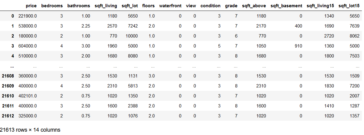

4 Data pre-processing

4.1 Determination of the predictors and the criterion

x = df.drop('price', axis=1)
y = df['price']

4.2 Train-Validation-Test Split

In the following, I will randomly assign 70% of the data to the training part and 15% each to the validation and test part.

train_ratio = 0.70
validation_ratio = 0.15
test_ratio = 0.15

# Generate TrainX and TrainY
trainX, testX, trainY, testY = train_test_split(x, y, test_size= 1 - train_ratio)
# Genearate ValX, TestX, ValY and TestY
valX, testX, valY, testY = train_test_split(testX, testY, test_size=test_ratio/(test_ratio + validation_ratio))

print(trainX.shape)
print(valX.shape)
print(testX.shape)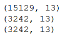

4.3 Scaling

sc=StandardScaler()

scaler = sc.fit(trainX)

trainX_scaled = scaler.transform(trainX)
valX_scaled = scaler.transform(valX)
testX_scaled = scaler.transform(testX)

5 ANN for Regression

5.1 Name Definitions

checkpoint_no = 'ckpt_1_ANN'
model_name = 'House_ANN_2FC_F64_64_epoch_120'

5.2 Parameter Settings

input_shape = trainX.shape[1]

n_batch_size = 128

n_steps_per_epoch = int(trainX.shape[0] / n_batch_size)
n_validation_steps = int(valX.shape[0] / n_batch_size)
n_test_steps = int(testX.shape[0] / n_batch_size)

n_epochs = 120


print('Input Shape: ' + str(input_shape))
print('Batch Size: ' + str(n_batch_size))
print()
print('Steps per Epoch: ' + str(n_steps_per_epoch))
print()
print('Validation Steps: ' + str(n_validation_steps))
print('Test Steps: ' + str(n_test_steps))
print()
print('Number of Epochs: ' + str(n_epochs))

5.3 Layer Structure

model = models.Sequential()
model.add(layers.Dense(64, activation='relu', input_shape=(input_shape,)))
model.add(layers.Dense(64, activation='relu'))
model.add(layers.Dense(1))

model.summary()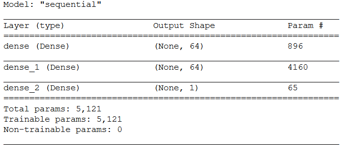

5.4 Configuring the model for training

model.compile(loss='mse',
              optimizer='rmsprop',
              metrics=['mae'])

5.5 Callbacks

If you want to know more about callbacks you can read about it here at Keras or also in my post about Convolutional Neural Networks.

# Prepare a directory to store all the checkpoints.
checkpoint_dir = './'+ checkpoint_no
if not os.path.exists(checkpoint_dir):
    os.makedirs(checkpoint_dir)

keras_callbacks = [ModelCheckpoint(filepath = checkpoint_dir + '/' + model_name, 
                                   monitor='val_loss', save_best_only=True, mode='auto')]

5.6 Fitting the model

history = model.fit(trainX_scaled,
                    trainY,
                    steps_per_epoch=n_steps_per_epoch,
                    epochs=n_epochs,
                    batch_size=n_batch_size,
                    validation_data=(valX_scaled, valY),
                    validation_steps=n_validation_steps,
                    callbacks=[keras_callbacks])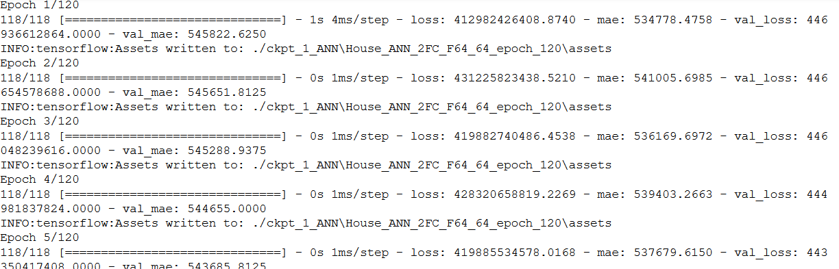

5.7 Obtaining the best model values

hist_df = pd.DataFrame(history.history)
hist_df['epoch'] = hist_df.index + 1
cols = list(hist_df.columns)
cols = [cols[-1]] + cols[:-1]
hist_df = hist_df[cols]
hist_df.to_csv(checkpoint_no + '/' + 'history_df_' + model_name + '.csv')
hist_df.head()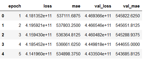

values_of_best_model = hist_df[hist_df.val_loss == hist_df.val_loss.min()]
values_of_best_model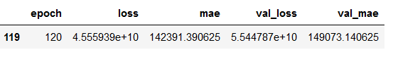

5.8 Storing all necessary metrics

After we have used the StandardScaler in chapter 4.3, we should also save it for later use.

pk.dump(scaler, open(checkpoint_no + '/' + 'scaler.pkl', 'wb'))

5.9 Validation

What the following metrics mean and how to interpret them I have described in the following post: Metrics for Regression Analysis

5.9.1 Metrics from model training (history)

mae = history.history['mae']
val_mae = history.history['val_mae']
loss = history.history['loss']
val_loss = history.history['val_loss']

epochs = range(1, len(mae) + 1)

plt.plot(epochs, mae, 'bo', label='Training MAE')
plt.plot(epochs, val_mae, 'b', label='Validation MAE')
plt.title('Training and validation MAE')
plt.legend()

plt.figure()

plt.plot(epochs, loss, 'bo', label='Training loss')
plt.plot(epochs, val_loss, 'b', label='Validation loss')
plt.title('Training and validation loss')
plt.legend()

plt.show()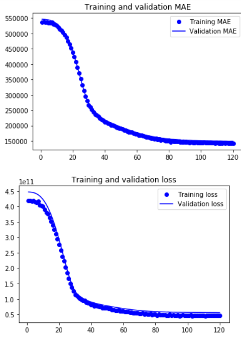

5.9.2 K-fold cross validation

In the following, I will perform cross-validation for the selected layer structure (chapter 5.3) and the specified parameter (chapter 5.2). The cross-validation is performed on the trainX_scaled and trainY parts, since the metrics from the model training (chapter 5.9.1) were also created based only on these data and the test part remains untouched until the end.

5.9.2.1 Determination of the layer structure as well as the number of cross-validations

In order to be able to validate the layered structure defined in chapter 5.3 in a meaningful way, the same structure must of course also be used here. The same applies to the parameters defined in chapter 5.2.

def build_model():
    model = models.Sequential()
    model.add(layers.Dense(64, activation='relu',
                           input_shape=(input_shape,)))
    model.add(layers.Dense(64, activation='relu'))
    model.add(layers.Dense(1))
    model.compile(loss='mse', optimizer='rmsprop', metrics=['mae'])
    return model

Here we only define the number of cross validations that should be performed.

k = 5
num_val_samples = len(trainX) // k

5.9.2.2 Obtaining the MAE for each fold

Here, each MAE for each fold is stored in all_scores.

all_scores = []
for i in range(k):
    print('Processing Fold', i)
    val_data = trainX_scaled[i * num_val_samples: (i + 1) * num_val_samples]
    val_targets = trainY[i * num_val_samples: (i + 1) * num_val_samples]

    partial_train_data = np.concatenate(
        [trainX_scaled[:i * num_val_samples],
         trainX_scaled[(i + 1) * num_val_samples:]],
        axis=0)
    partial_train_targets = np.concatenate(
        [trainY[:i * num_val_samples],
         trainY[(i + 1) * num_val_samples:]],
        axis=0)

    model = build_model()
    model.fit(partial_train_data, partial_train_targets,
              epochs=n_epochs, batch_size=n_batch_size, verbose=0)
    val_mse, val_mae = model.evaluate(val_data, val_targets, verbose=0)
    all_scores.append(val_mae)
    print('MAE: ' + str(val_mae))
    print('----------------------')

for i, val in enumerate(all_scores):
    print('Fold ' + str(i) +': ' + 'MAE of', val)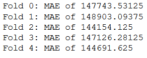

print('Mean MAE of all folds: ' + str(np.mean(all_scores)))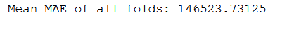

5.9.2.3 Obtaining the MAE for each epoch

Here, each MAE of each step for each epoch for each epoch is stored in all_mae_histories.

all_mae_histories = []
for i in range(k):
    print('Processing Fold', i)
    val_data = trainX_scaled[i * num_val_samples: (i + 1) * num_val_samples]
    val_targets = trainY[i * num_val_samples: (i + 1) * num_val_samples]
    partial_train_data = np.concatenate(
        [trainX_scaled[:i * num_val_samples],
         trainX_scaled[(i + 1) * num_val_samples:]],
        axis=0)
    partial_train_targets = np.concatenate(
        [trainY[:i * num_val_samples],
         trainY[(i + 1) * num_val_samples:]],
        axis=0)

    model = build_model()
    history = model.fit(partial_train_data, partial_train_targets,
                        validation_data=(val_data, val_targets),
                        epochs=n_epochs, batch_size=n_batch_size, verbose=0)
    mae_history = history.history['val_mae']
    all_mae_histories.append(mae_history)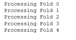

Here we now calculate the average MAE achieved per epoch.

average_mae_history = [np.mean([x[i] for x in all_mae_histories]) for i in range(n_epochs)]

len(average_mae_history)

plt.plot(range(1, len(average_mae_history) + 1), average_mae_history)
plt.title('Validation MAE per Epoch')
plt.xlabel('Epochs')
plt.ylabel('Validation MAE')
plt.show()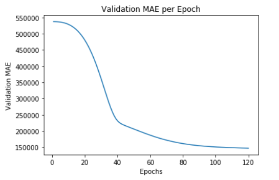

With real-world data, we often get messy curves. Here the following function can help:

def smooth_curve(points, factor=0.9):
      '''
      Function for smoothing data points

      Args:
          points (float64): Array of floats to be smoothed, numpy array of floats

      Returns:
          Smoothed data points
      '''  
      smoothed_points = []
      for point in points:
        if smoothed_points:
          previous = smoothed_points[-1]
          smoothed_points.append(previous * factor + point * (1 - factor))
        else:
          smoothed_points.append(point)
      return smoothed_points

Here we also have the option to exclude the first n values from the graph. So that the graphic does not become misleading with regard to the displayed epochs, I change the index accordingly before I create the plot.

n_first_observations_to_exclude = 30

smooth_mae_history = smooth_curve(average_mae_history[n_first_observations_to_exclude:])

smooth_mae_history = pd.DataFrame(smooth_mae_history)
smooth_mae_history = smooth_mae_history.set_index(smooth_mae_history.index + n_first_observations_to_exclude)
smooth_mae_history.head()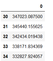

plt.plot(smooth_mae_history)
plt.title('Validation MAE per Epoch')
plt.xlabel('Epochs')
plt.ylabel('Validation MAE')
plt.show()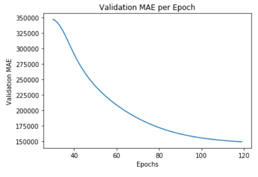

5.10 Load best model

Again, reference to the Computer Vision posts where I explained why and how I cleaned up the Model Checkpoint folders.

# Loading the automatically saved model
model_reloaded = load_model(checkpoint_no + '/' + model_name)

# Saving the best model in the correct path and format
root_directory = os.getcwd()
checkpoint_dir = os.path.join(root_directory, checkpoint_no)
model_name_temp = os.path.join(checkpoint_dir, model_name + '.h5')
model_reloaded.save(model_name_temp)

# Deletion of the automatically created folder under Model Checkpoint File.
folder_name_temp = os.path.join(checkpoint_dir, model_name)
shutil.rmtree(folder_name_temp, ignore_errors=True)

best_model = load_model(model_name_temp)

The overall folder structure should look like this:

5.11 Model Testing

test_loss, test_mae = best_model.evaluate(testX_scaled,
                                          testY,
                                          steps=n_test_steps)
print()
print('Test MAE:', test_mae)

5.12 Predictions

y_pred = model.predict(testX_scaled)
y_pred[:5]

5.13 Evaluation

df_testY = pd.DataFrame(testY)
df_y_pred = pd.DataFrame(y_pred)

df_testY.reset_index(drop=True, inplace=True)
df_y_pred.reset_index(drop=True, inplace=True)

df_results = pd.concat([df_testY, df_y_pred], axis=1)
df_results.columns = ['Actual', 'Predicted']

df_results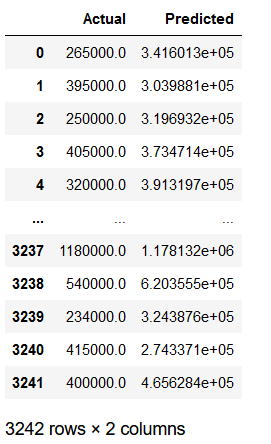

print('Mean Absolute Error:', metrics.mean_absolute_error(testY, y_pred))
print('Mean Squared Error:', metrics.mean_squared_error(testY, y_pred))
print('Root Mean Squared Error:', metrics.mean_squared_error(testY, y_pred, squared=False))
print('Mean Absolute Percentage Error:', metrics.mean_absolute_percentage_error(testY, y_pred))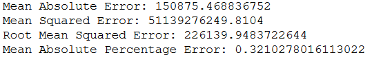

Now why is this designated MAE (150875) larger than the test MAE (147006)?

This is because when we test MAE with the .evaluate() function, we go through multiple steps (25 in this case) and a separate MAE is calculated for each. On average we get a MAE of 147006 with the .evaluate() function.

6 Prevent Overfitting

At this point I would like to remind you of the topic of overfitting. In my post (Artificial Neural Network for binary Classification) I explained in more detail what can be done against overfitting. Here again a list with the corresponding links:

7 Conclusion

Again, as a reminder which metrics should be stored additionally when using neural networks in real life:

Mean values of the individual predictors in order to be able to compensate for missing values later on.
Encoders for predictors, if categorical features are converted.
If variables would have been excluded, a list with the final features should have been stored.

For what reason I give these recommendations can be well read in my Data Science Post. Here I have also created best practice guidelines on how to proceed with model training.

References

The content of the entire post was created using the following sources:

Chollet, F. (2018). Deep learning with Python (Vol. 361). New York: Manning.

NN - Artificial Neural Network for Regression Analysis