1 Introduction

As announced in my last post, I will now create a neural network using a Deep Learning library (Keras in this case) to solve binary classification problems.

For this publication the dataset Winequality from the statistic platform “Kaggle” was used. You can download it from my “GitHub Repository”.

2 Loading the libraries

import pandas as pd
import os
import shutil
import pickle as pk
import matplotlib.pyplot as plt

from sklearn.preprocessing import LabelEncoder
from sklearn.model_selection import train_test_split

from keras import models
from keras import layers
from keras.callbacks import EarlyStopping, ModelCheckpoint
from keras.models import load_model

3 Loading the data

df = pd.read_csv('winequality.csv').dropna()
df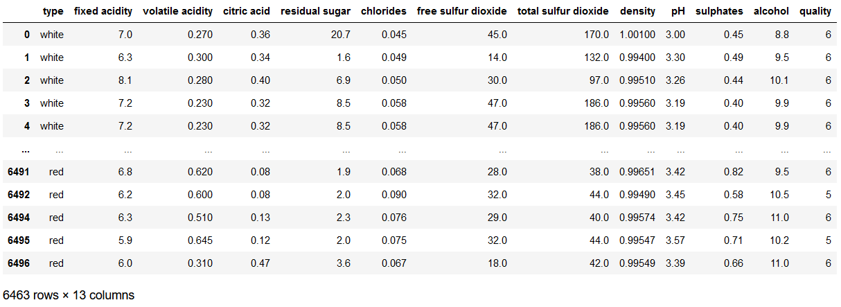

df['type'].value_counts()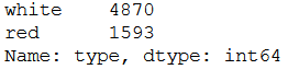

4 Data pre-processing

4.1 Determination of the predictors and the criterion

x = df.drop('type', axis=1)
y = df['type']

4.2 Encoding

Since all variables must be numeric, we must recode the criterion at this point. For this I used the LabelEncoder. How to use it can be read in the following post: Types of Encoder

encoder = LabelEncoder()

encoded_Y = encoder.fit_transform(y)
encoded_Y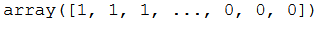

4.3 Train-Validation-Test Split

As already known from the computer vision posts, for neural networks we need to split our dataset into a training part, a validation part and a testing part. In the following, I will randomly assign 70% of the data to the training part and 15% each to the validation and test part.

train_ratio = 0.70
validation_ratio = 0.15
test_ratio = 0.15

# Generate TrainX and TrainY
trainX, testX, trainY, testY = train_test_split(x, encoded_Y, test_size= 1 - train_ratio)
# Genearate ValX, TestX, ValY and TestY
valX, testX, valY, testY = train_test_split(testX, testY, test_size=test_ratio/(test_ratio + validation_ratio))

print(trainX.shape)
print(valX.shape)
print(testX.shape)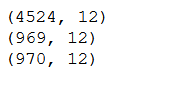

5 ANN for binary Classification

My approach to using neural networks with Keras is described in detail in my post Computer Vision - Convolutional Neural Network and can be read there if something is unclear.

5.1 Name Definitions

checkpoint_no = 'ckpt_1_ANN'
model_name = 'Wine_ANN_2FC_F16_16_epoch_25'

5.2 Parameter Settings

input_shape = trainX.shape[1]

n_batch_size = 100

n_steps_per_epoch = int(trainX.shape[0] / n_batch_size)
n_validation_steps = int(valX.shape[0] / n_batch_size)
n_test_steps = int(testX.shape[0] / n_batch_size)

n_epochs = 25


print('Input Shape: ' + str(input_shape))
print('Batch Size: ' + str(n_batch_size))
print()
print('Steps per Epoch: ' + str(n_steps_per_epoch))
print()
print('Validation Steps: ' + str(n_validation_steps))
print('Test Steps: ' + str(n_test_steps))
print()
print('Number of Epochs: ' + str(n_epochs))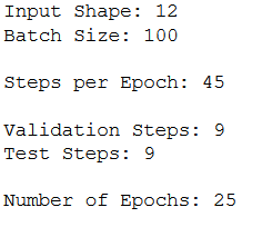

5.3 Layer Structure

model = models.Sequential()
model.add(layers.Dense(16, activation='relu', input_shape=(input_shape,)))
model.add(layers.Dense(16, activation='relu'))
model.add(layers.Dense(1, activation='sigmoid'))

model.summary()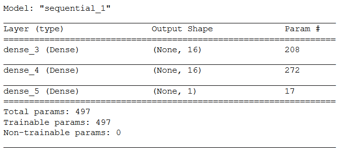

5.4 Configuring the model for training

model.compile(loss='binary_crossentropy',
              optimizer='adam',
              metrics=['accuracy'])

5.5 Callbacks

If you want to know more about callbacks you can read about it here at Keras or also in my post about Convolutional Neural Networks.

# Prepare a directory to store all the checkpoints.
checkpoint_dir = './'+ checkpoint_no
if not os.path.exists(checkpoint_dir):
    os.makedirs(checkpoint_dir)

keras_callbacks = [ModelCheckpoint(filepath = checkpoint_dir + '/' + model_name, 
                                   monitor='val_loss', save_best_only=True, mode='auto')]

5.6 Fitting the model

history = model.fit(trainX,
                    trainY,
                    steps_per_epoch=n_steps_per_epoch,
                    epochs=n_epochs,
                    batch_size=n_batch_size,
                    validation_data=(valX, valY),
                    validation_steps=n_validation_steps,
                    callbacks=[keras_callbacks])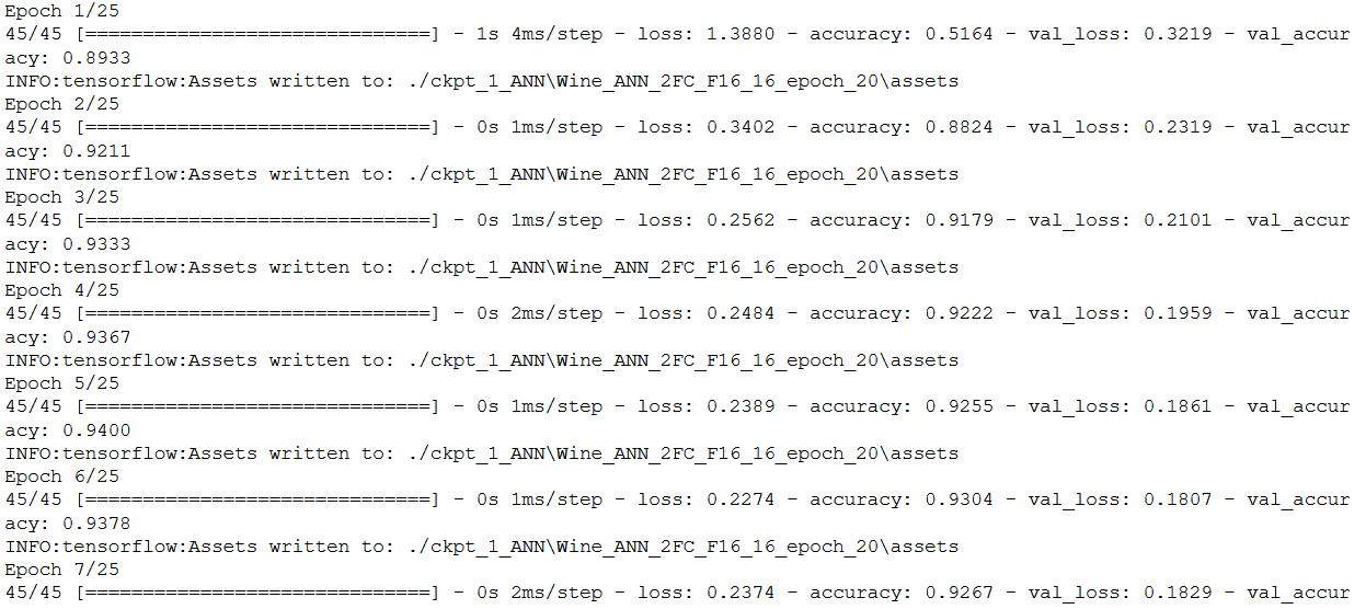

5.7 Obtaining the best model values

hist_df = pd.DataFrame(history.history)
hist_df['epoch'] = hist_df.index + 1
cols = list(hist_df.columns)
cols = [cols[-1]] + cols[:-1]
hist_df = hist_df[cols]
hist_df.to_csv(checkpoint_no + '/' + 'history_df_' + model_name + '.csv')
hist_df.head()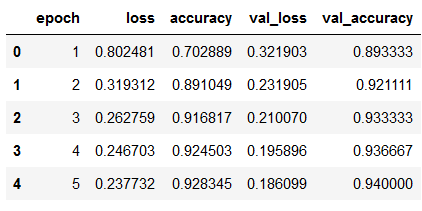

values_of_best_model = hist_df[hist_df.val_loss == hist_df.val_loss.min()]
values_of_best_model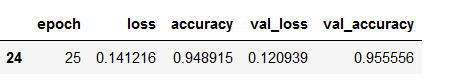

5.8 Obtaining class assignments

Similar to the neural networks for computer vision, I also save the class assignments for later reuse.

class_assignment = dict(zip(y, encoded_Y))

df_temp = pd.DataFrame([class_assignment], columns=class_assignment.keys())
df_temp = df_temp.stack()
df_temp = pd.DataFrame(df_temp).reset_index().drop(['level_0'], axis=1)
df_temp.columns = ['Category', 'Allocated Number']
df_temp.to_csv(checkpoint_no + '/' + 'class_assignment_df_' + model_name + '.csv')

print('Class assignment:', str(class_assignment))

The encoder used is also saved.

pk.dump(encoder, open(checkpoint_no + '/' + 'encoder.pkl', 'wb'))

5.9 Validation

acc = history.history['accuracy']
val_acc = history.history['val_accuracy']
loss = history.history['loss']
val_loss = history.history['val_loss']

epochs = range(1, len(acc) + 1)

plt.plot(epochs, acc, 'bo', label='Training acc')
plt.plot(epochs, val_acc, 'b', label='Validation acc')
plt.title('Training and validation accuracy')
plt.legend()

plt.figure()

plt.plot(epochs, loss, 'bo', label='Training loss')
plt.plot(epochs, val_loss, 'b', label='Validation loss')
plt.title('Training and validation loss')
plt.legend()

plt.show()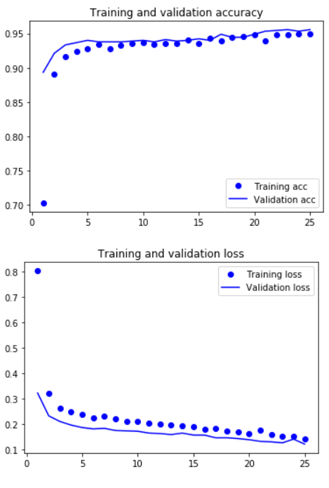

5.10 Load best model

Again, reference to the Computer Vision posts where I explained why and how I cleaned up the Model Checkpoint folders.

# Loading the automatically saved model
model_reloaded = load_model(checkpoint_no + '/' + model_name)

# Saving the best model in the correct path and format
root_directory = os.getcwd()
checkpoint_dir = os.path.join(root_directory, checkpoint_no)
model_name_temp = os.path.join(checkpoint_dir, model_name + '.h5')
model_reloaded.save(model_name_temp)

# Deletion of the automatically created folder under Model Checkpoint File.
folder_name_temp = os.path.join(checkpoint_dir, model_name)
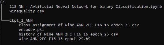
shutil.rmtree(folder_name_temp, ignore_errors=True)

best_model = load_model(model_name_temp)

The overall folder structure should look like this:

5.11 Model Testing

test_loss, test_acc = best_model.evaluate(testX,
                                          testY,
                                          steps=n_test_steps)
print()
print('Test Accuracy:', test_acc)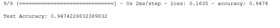

5.12 Predictions

y_pred = model.predict(testX)
y_pred

6 Prevent Overfitting

Often you have the problem of overfitting. For this reason, I have presented here a few approaches on how to counteract overfitting.

6.1 Original Layer Structure

Here again, as a reminder, the used layer structure:

model = models.Sequential()
model.add(layers.Dense(16, activation='relu', input_shape=(input_shape,)))
model.add(layers.Dense(16, activation='relu'))
model.add(layers.Dense(1, activation='sigmoid'))

6.2 Reduce the network’s size

The first thing I always try to do is to change something in the layer structure. To counteract overfitting, it is often advisable to reduce the layer structure. Using our example, I would try the following new layer structure if overfitting existed.

model = models.Sequential()
model.add(layers.Dense(4, activation='relu', input_shape=(input_shape,)))
model.add(layers.Dense(4, activation='relu'))
model.add(layers.Dense(1, activation='sigmoid'))

6.3 Adding weight regularization

Another option is Weight Regularization:

from keras import regularizers

model = models.Sequential()
model.add(layers.Dense(16, kernel_regularizer=regularizers.l2(0.001),
                       activation='relu', input_shape=(input_shape,)))
model.add(layers.Dense(16, kernel_regularizer=regularizers.l2(0.001),
                       activation='relu'))
model.add(layers.Dense(1, activation='sigmoid'))

6.4 Adding dropout

As I used to do with Computer Vision, adding dropout layers is also a very useful option.

An example layer structure in our case would look like this:

model = models.Sequential()
model.add(layers.Dense(16, activation='relu', input_shape=(input_shape,)))
model.add(layers.Dropout(0.5))
model.add(layers.Dense(16, activation='relu'))
model.add(layers.Dropout(0.5))
model.add(layers.Dense(1, activation='sigmoid'))

7 Conclusion

Lastly, I would like to mention a few points regarding this post. It was not relevant for this dataset but in case it was (and with real world data this is mostly the case) further metrics should be stored:

Mean values of the individual predictors in order to be able to compensate for missing values later on.
Further encoders for predictors, if categorical features are converted.
Scaler, if these are used.
If variables would have been excluded, a list with the final features should have been stored.

For what reason I give these recommendations can be well read in my Data Science Post. Here I have also created best practice guidelines on how to proceed with model training.

I would like to add one limitation at this point. You may have noticed it already, but the dataset was heavily imbalanced. How to deal with such problems I have explained here: Dealing with imbalanced classes

References

The content of the entire post was created using the following sources:

Chollet, F. (2018). Deep learning with Python (Vol. 361). New York: Manning.

NN – Artificial Neural Network for binary Classification