1 Introduction

In my last post, I showed how to do binary classification using the Keras deep learning library. Now I would like to show how to make multi-class classifications.

For this publication the dataset bird from the statistic platform “Kaggle” was used. You can download it from my “GitHub Repository”.

2 Loading the libraries

import pandas as pd
import numpy as np
import os
import shutil
import pickle as pk
import matplotlib.pyplot as plt

from sklearn.preprocessing import OneHotEncoder
from sklearn.model_selection import train_test_split

from keras import models
from keras import layers
from keras.callbacks import EarlyStopping, ModelCheckpoint
from keras.models import load_model

3 Loading the data

df = pd.read_csv('bird.csv').dropna()

print()
print('Shape of dataframe:')
print(str(df.shape))
print()
print('Head of dataframe:')
df.head()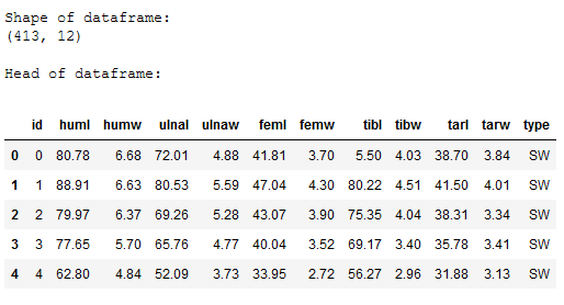

Description of predictors:

Length and Diameter of Humerus
Length and Diameter of Ulna
Length and Diameter of Femur
Length and Diameter of Tibiotarsus
Length and Diameter of Tarsometatarsus

df['type'].value_counts()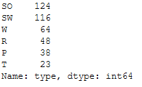

Description of the target variable:

SW: Swimming Birds
W: Wading Birds
T: Terrestrial Birds
R: Raptors
P: Scansorial Birds
SO: Singing Birds

4 Data pre-processing

4.1 Determination of the predictors and the criterion

x = df.drop('type', axis=1)
y = df['type']

4.2 Encoding

Last time (Artificial Neural Network for binary Classification) we used LabelEncoder for this. Since we now want to do a multi-class classification we need One-Hot Encoding.

encoder = OneHotEncoder()

encoded_Y = encoder.fit(y.values.reshape(-1,1))
encoded_Y = encoded_Y.transform(y.values.reshape(-1,1)).toarray()

encoded_Y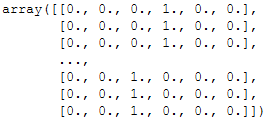

4.3 Train-Validation-Test Split

In the following, I will randomly assign 70% of the data to the training part and 15% each to the validation and test part.

train_ratio = 0.70
validation_ratio = 0.15
test_ratio = 0.15

# Generate TrainX and TrainY
trainX, testX, trainY, testY = train_test_split(x, encoded_Y, test_size= 1 - train_ratio)
# Genearate ValX, TestX, ValY and TestY
valX, testX, valY, testY = train_test_split(testX, testY, test_size=test_ratio/(test_ratio + validation_ratio))

print(trainX.shape)
print(valX.shape)
print(testX.shape)

4.4 Check if all classes are included in every split part

Since this is a very small dataset with 413 observations and the least represented class contains only 23 observations, I advise at this point to check whether all classes are included in the variables created by the train validation test split.

re_transformed_array_trainY = encoder.inverse_transform(trainY)

unique_elements, counts_elements = np.unique(re_transformed_array_trainY, return_counts=True)
unique_elements_and_counts_trainY = pd.DataFrame(np.asarray((unique_elements, counts_elements)).T)
unique_elements_and_counts_trainY.columns = ['unique_elements', 'count']

unique_elements_and_counts_trainY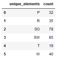

re_transformed_array_valY = encoder.inverse_transform(valY)

unique_elements, counts_elements = np.unique(re_transformed_array_valY, return_counts=True)
unique_elements_and_counts_valY = pd.DataFrame(np.asarray((unique_elements, counts_elements)).T)
unique_elements_and_counts_valY.columns = ['unique_elements', 'count']

unique_elements_and_counts_valY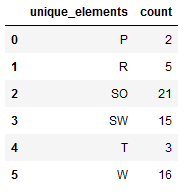

re_transformed_array_testY = encoder.inverse_transform(testY)

unique_elements, counts_elements = np.unique(re_transformed_array_testY, return_counts=True)
unique_elements_and_counts_testY = pd.DataFrame(np.asarray((unique_elements, counts_elements)).T)
unique_elements_and_counts_testY.columns = ['unique_elements', 'count']

unique_elements_and_counts_testY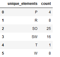

Of course, you can also use a for-loop:

y_part = [trainY, valY, testY]

for y_part in y_part:
    re_transformed_array = encoder.inverse_transform(y_part)
    
    unique_elements, counts_elements = np.unique(re_transformed_array, return_counts=True)
    unique_elements_and_counts = pd.DataFrame(np.asarray((unique_elements, counts_elements)).T)
    unique_elements_and_counts.columns = ['unique_elements', 'count']
    print('---------------')
    print(unique_elements_and_counts)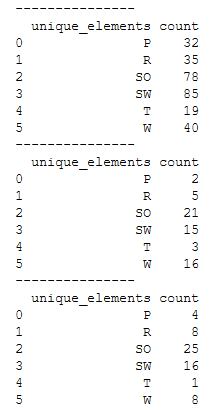

To check if all categories are contained in all three variables (trainY, valY and testY) I first store the unique elements in lists and can then compare them with a logical query.

list_trainY = unique_elements_and_counts_trainY['unique_elements'].to_list()
list_valY = unique_elements_and_counts_valY['unique_elements'].to_list()
list_testY = unique_elements_and_counts_testY['unique_elements'].to_list()

print(list_trainY)
print(list_valY)
print(list_testY)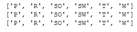

check_val =  all(item in list_valY for item in list_trainY)
 
if check_val is True:
    print('OK !')
    print("The list_valY contains all elements of the list_trainY.")    
else :
    print()
    print('No !')
    print("List_valY doesn't have all elements of the list_trainY.")

check_test =  all(item in list_testY for item in list_trainY)
 
if check_test is True:
    print('OK !')
    print("The list_testY contains all elements of the list_trainY.")    
else :
    print()
    print('No !')
    print("List_testY doesn't have all elements of the list_trainY.")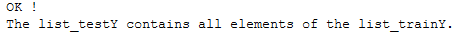

5 ANN for Multi-Class Classfication

5.1 Name Definitions

checkpoint_no = 'ckpt_1_ANN'
model_name = 'Bird_ANN_2FC_F64_64_epoch_25'

5.2 Parameter Settings

input_shape = trainX.shape[1]

n_batch_size = 20

n_steps_per_epoch = int(trainX.shape[0] / n_batch_size)
n_validation_steps = int(valX.shape[0] / n_batch_size)
n_test_steps = int(testX.shape[0] / n_batch_size)

n_epochs = 25

num_classes = trainY.shape[1]

print('Input Shape: ' + str(input_shape))
print('Batch Size: ' + str(n_batch_size))
print()
print('Steps per Epoch: ' + str(n_steps_per_epoch))
print()
print('Validation Steps: ' + str(n_validation_steps))
print('Test Steps: ' + str(n_test_steps))
print()
print('Number of Epochs: ' + str(n_epochs))
print()
print('Number of Classes: ' + str(num_classes))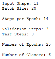

5.3 Layer Structure

Here I use the activation function ‘softmax’ in contrast to the binary classification.

model = models.Sequential()
model.add(layers.Dense(64, activation='relu', input_shape=(input_shape,)))
model.add(layers.Dense(64, activation='relu'))
model.add(layers.Dense(num_classes, activation='softmax'))

model.summary()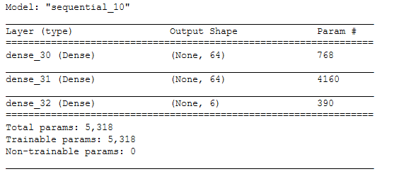

5.4 Configuring the model for training

Again, the neural network for multi-class classification differs from that for binary classification. Here the loss function ‘categorical_crossentropy’ is used.

model.compile(loss='categorical_crossentropy',
              optimizer='adam',
              metrics=['accuracy'])

5.5 Callbacks

If you want to know more about callbacks you can read about it here at Keras or also in my post about Convolutional Neural Networks.

# Prepare a directory to store all the checkpoints.
checkpoint_dir = './'+ checkpoint_no
if not os.path.exists(checkpoint_dir):
    os.makedirs(checkpoint_dir)

keras_callbacks = [ModelCheckpoint(filepath = checkpoint_dir + '/' + model_name, 
                                   monitor='val_loss', save_best_only=True, mode='auto')]

5.6 Fitting the model

history = model.fit(trainX,
                    trainY,
                    steps_per_epoch=n_steps_per_epoch,
                    epochs=n_epochs,
                    batch_size=n_batch_size,
                    validation_data=(valX, valY),
                    validation_steps=n_validation_steps,
                    callbacks=[keras_callbacks])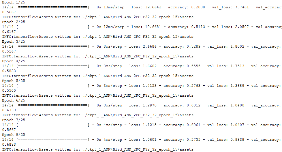

5.7 Obtaining the best model values

hist_df = pd.DataFrame(history.history)
hist_df['epoch'] = hist_df.index + 1
cols = list(hist_df.columns)
cols = [cols[-1]] + cols[:-1]
hist_df = hist_df[cols]
hist_df.to_csv(checkpoint_no + '/' + 'history_df_' + model_name + '.csv')
hist_df.head()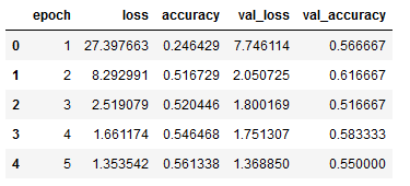

values_of_best_model = hist_df[hist_df.val_loss == hist_df.val_loss.min()]
values_of_best_model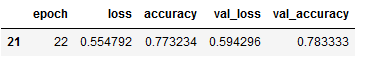

5.8 Obtaining class assignments

Similar to the neural networks for computer vision, I also save the class assignments for later reuse.

class_assignment = dict(zip(y, encoded_Y))

df_temp = pd.DataFrame([class_assignment], columns=class_assignment.keys())
df_temp = df_temp.stack()
df_temp = pd.DataFrame(df_temp).reset_index().drop(['level_0'], axis=1)
df_temp.columns = ['Category', 'Allocated Number']

df_temp.to_csv(checkpoint_no + '/' + 'class_assignment_df_' + model_name + '.csv')

print('Class assignment:')
class_assignment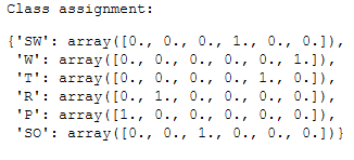

The encoder used is also saved.

pk.dump(encoder, open(checkpoint_no + '/' + 'encoder.pkl', 'wb'))

5.9 Validation

acc = history.history['accuracy']
val_acc = history.history['val_accuracy']
loss = history.history['loss']
val_loss = history.history['val_loss']

epochs = range(1, len(acc) + 1)

plt.plot(epochs, acc, 'bo', label='Training acc')
plt.plot(epochs, val_acc, 'b', label='Validation acc')
plt.title('Training and validation accuracy')
plt.legend()

plt.figure()

plt.plot(epochs, loss, 'bo', label='Training loss')
plt.plot(epochs, val_loss, 'b', label='Validation loss')
plt.title('Training and validation loss')
plt.legend()

plt.show()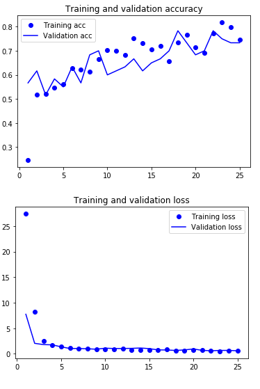

5.10 Load best model

Again, reference to the Computer Vision posts where I explained why and how I cleaned up the Model Checkpoint folders.

# Loading the automatically saved model
model_reloaded = load_model(checkpoint_no + '/' + model_name)

# Saving the best model in the correct path and format
root_directory = os.getcwd()
checkpoint_dir = os.path.join(root_directory, checkpoint_no)
model_name_temp = os.path.join(checkpoint_dir, model_name + '.h5')
model_reloaded.save(model_name_temp)

# Deletion of the automatically created folder under Model Checkpoint File.
folder_name_temp = os.path.join(checkpoint_dir, model_name)
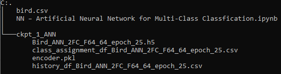
shutil.rmtree(folder_name_temp, ignore_errors=True)

best_model = load_model(model_name_temp)

The overall folder structure should look like this:

5.11 Model Testing

test_loss, test_acc = best_model.evaluate(testX,
                                          testY,
                                          steps=n_test_steps)
print()
print('Test Accuracy:', test_acc)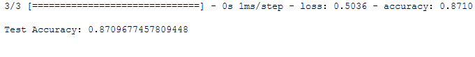

5.12 Predictions

Now it’s time for some predictions. Here I printed the first 5 results.

y_pred = model.predict(testX)
y_pred[:5]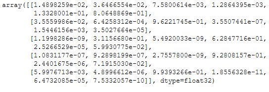

Now we need the previously saved encoder to recode the data.

encoder_reload = pk.load(open(checkpoint_dir + '\\' + 'encoder.pkl','rb'))

re_transformed_y_pred = encoder_reload.inverse_transform(y_pred)
re_transformed_y_pred[:5]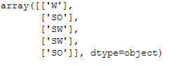

Now we can see which bird species was predicted. If you want the result to be even more beautiful, you can add the predicted values to the testX part:

testX['re_transformed_y_pred'] = re_transformed_y_pred
testX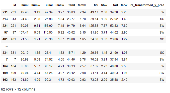

6 Prevent Overfitting

At this point I would like to remind you of the topic of overfitting. In my last post (Artificial Neural Network for binary Classification) I explained in more detail what can be done against overfitting. Here again a list with the corresponding links:

7 Conclusion

Again, as a reminder which metrics should be stored additionally when using neural networks in real life:

Mean values of the individual predictors in order to be able to compensate for missing values later on.
Further encoders for predictors, if categorical features are converted.
Scaler, if these are used.
If variables would have been excluded, a list with the final features should have been stored.

For what reason I give these recommendations can be well read in my Data Science Post. Here I have also created best practice guidelines on how to proceed with model training.

I would like to add one limitation at this point. You may have noticed it already, but the dataset was heavily imbalanced. How to deal with such problems I have explained here: Dealing with imbalanced classes

References

The content of the entire post was created using the following sources:

Chollet, F. (2018). Deep learning with Python (Vol. 361). New York: Manning.

NN – Artificial Neural Network for Multi-Class Classfication