- 1 Introduction
- 2 Import the libraries
- 3 Import the data
- 4 Answering Research Questions - Descriptive Statistics
- 5 Development of a Machine Learning Model End to End Process
- 6 Conclusion
- 7 Data Science Best Practice Guidlines for ML-Model Development
- 8 Limitations
1 Introduction
With reference to my project in the “Data Science Nanodegree” of “Udacity” I would like to show the Data Science Process according to CRISP-DM. If you are interested in the exact content of this course look “here”.
For this post the dataset house-prices from the statistic platform “Kaggle” was used. A copy of the record is available at my “GitHub Repo”.
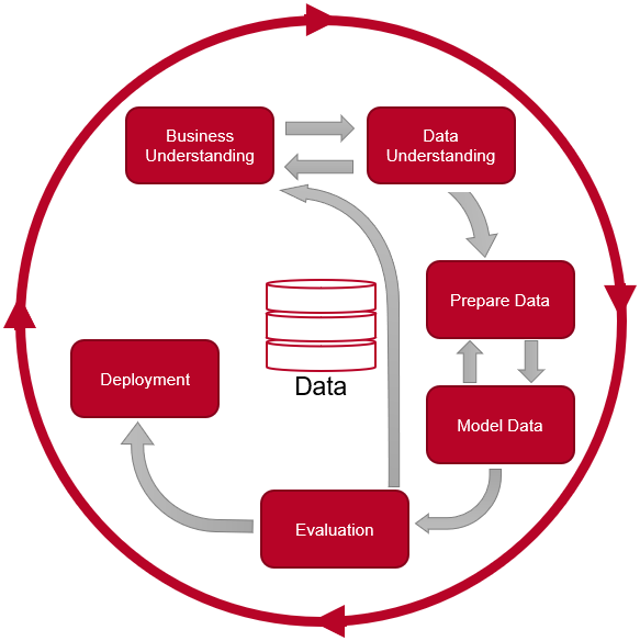
CRISP-DM
CRISP-DM stands for Cross Industry Standard Process for Data Mining and describes the six phases in a data mining project.
- Phase 1 Business Understanding:
In the business understanding phase, it is important to define the concrete goals and requirements for data mining. The result of this phase is the formulation of the task and the description of the planned rough procedure.
- Phase 2 Data Understanding:
In the context of data understanding, an attempt is made to gain an initial overview of the available data and its quality. An analysis and evaluation of the data quality is carried out. Problems with the quality of the available data in relation to the tasks defined in the previous phase must be identified.
- Phase 3 Data Preparation:
The purpose of data preparation is to create a final data set that forms the basis for the next phase of modeling.
- Phase 4 Modeling:
Within the scope of modeling, the data mining methods suitable for the task are applied to the data set created in the data preparation. Typical for this phase are the optimization of parameters and the creation of several models.
- Phase 5 Evaluation:
The evaluation ensures an exact comparison of the created data models with the task at hand and selects the most suitable model.
- Phase 6 Deployment:
The final phase of the CRISP-DM is the evaluation. In this phase, the obtained results are processed in order to present them and feed them into the decision process of the client.
In the following I will complete these 6 phases using real data. I will explain each of the steps in detail and explain why they are necessary and why I have done them this way.
2 Import the libraries
import pandas as pd
import numpy as np


from sklearn.preprocessing import LabelBinarizer
from sklearn.preprocessing import OneHotEncoder

import matplotlib.pyplot as plt
import seaborn as sns
sns.set()


from sklearn.cluster import KMeans
from sklearn.preprocessing import MinMaxScaler

import statsmodels.formula.api as smf

from sklearn.model_selection import train_test_split

import pickle as pk

from sklearn.preprocessing import StandardScaler

from sklearn.feature_selection import VarianceThreshold

from sklearn import metrics

from sklearn.feature_selection import RFE
from sklearn.linear_model import LinearRegression
3 Import the data
Here we get a first overview of the data available to us.
house_prices = pd.read_csv("house_prices_dataframe.csv")
house_prices.head()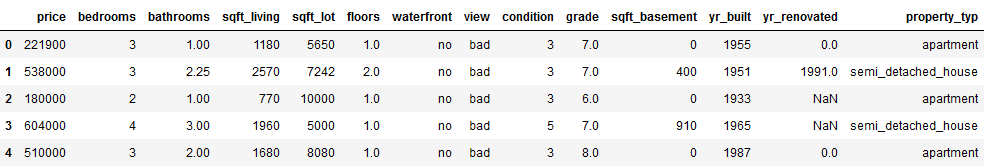
house_prices.shape
house_prices.dtypes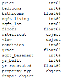
4 Answering Research Questions - Descriptive Statistics
The further procedure follows the Best Practice approach for ML Model Development. I have listed this approach at the end of this publication (chapter 7). It allows you to track the naming convention used and to see when which models, data sets or stored metrics are saved. You can also download these instructions here: “DS Best Practice Guidlines for ML Model Development”.
4.1 Data pre-processing
4.1.1 Check for Outliers
First we will check the data frame for some outliers. This step is necessary first, because otherwise replacing missing values would be negatively affected. Categorical variables are not considered by this step.
For the identification of outliers the z-score method is used.
In statistics, if a data distribution is approximately normal then about 68% of the data points lie within one standard deviation (sd) of the mean and about 95% are within two standard deviations, and about 99.7% lie within three standard deviations.
Therefore, if you have any data point that is more than 3 times the standard deviation, then those points are very likely to be outliers.
We are going to check observations above a sd of 3 and remove these as an outlier.
'''
Here I defined a function do identificate observations with an sd above 3.
'''

def outliers_z_score(df):
    threshold = 3

    mean = np.mean(df)
    std = np.std(df)
    z_scores = [(y - mean) / std for y in df]
    return np.where(np.abs(z_scores) > threshold)
For the further proceeding we just need numerical colunns.
my_list = ['int16', 'int32', 'int64', 'float16', 'float32', 'float64']
num_columns = list(house_prices.select_dtypes(include=my_list).columns)
numerical_columns = house_prices[num_columns]
numerical_columns.head(3)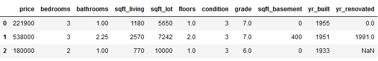
Now we are going to apply our outlier-function to all numerical columns
outlier_list = numerical_columns.apply(lambda x: outliers_z_score(x))
outlier_list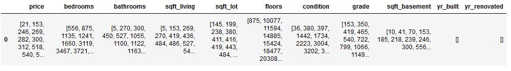
df_of_outlier = outlier_list.iloc[0]
df_of_outlier = pd.DataFrame(df_of_outlier)
df_of_outlier.columns = ['Rows_to_exclude']
df_of_outlier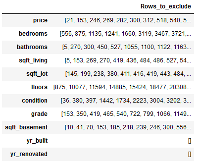
# Convert all values from column Rows_to_exclude to a numpy array
outlier_list_final = df_of_outlier['Rows_to_exclude'].to_numpy()

# Concatenate a whole sequence of arrays
outlier_list_final = np.concatenate( outlier_list_final, axis=0 )

# Drop dubplicate values
outlier_list_final_unique = set(outlier_list_final)
outlier_list_final_unique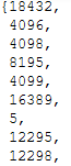
Now we are going to exclude the identified outliers from original dataframe.
filter_rows_to_exclude = house_prices.index.isin(outlier_list_final_unique)
df_without_outliers = house_prices[~filter_rows_to_exclude]
print('Length of original dataframe: ' + str(len(house_prices)))
print('Length of new dataframe without outliers: ' + str(len(df_without_outliers)))
print('----------------------------------------------------------------------------------------------------')
print('Difference between new and old dataframe: ' + str(len(house_prices) - len(df_without_outliers)))
print('----------------------------------------------------------------------------------------------------')
print('Length of unique outlier list: ' + str(len(outlier_list_final_unique)))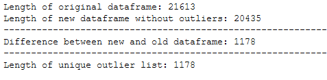
Important!
If you look at the index of the last two columns, you will notice that index 5 is missing. This is because the values from row 5 for the variables bathrooms and sqft_living were identified as outlier and removed accordingly.
The data set now has 1178 (the number of unique outliers) gaps at the corresponding position in the index. This can lead to problems if you want to join other tables via the index.
Since I know that this will be the case as soon as I encode the categorical variables, I proactively create a new index (via reset_index function) which will allow me to easily add new records later.
Below you can see the difference between index and new_index.
df_without_outliers = df_without_outliers.reset_index()

df_without_outliers = df_without_outliers.rename(columns={'index':'old_index'})

df_without_outliers.head(6)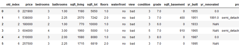
Here is a comparison of the distribution of values from the target variable ‘house price’ before and after outlier removal.
# Distribution before outlier removal
sns.boxplot(x='price', data=house_prices)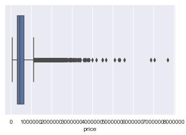
# Distribution after outlier removal
sns.boxplot(x='price', data=df_without_outliers)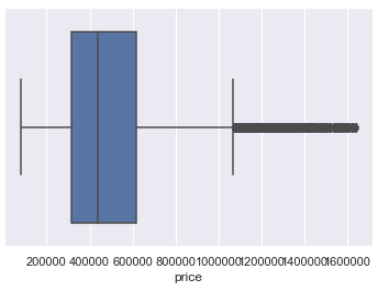
4.1.2 Check for Missing Values
Now we are going to check for missing values.
def missing_values_table(df):
        # Total missing values
        mis_val = df.isnull().sum()

        # Percentage of missing values
        mis_val_percent = 100 * df.isnull().sum() / len(df)

        # Make a table with the results
        mis_val_table = pd.concat([mis_val, mis_val_percent], axis=1)

        # Rename the columns
        mis_val_table_ren_columns = mis_val_table.rename(
        columns = {0 : 'Missing Values', 1 : '% of Total Values'})

        # Sort the table by percentage of missing descending
        mis_val_table_ren_columns = mis_val_table_ren_columns[
            mis_val_table_ren_columns.iloc[:,1] != 0].sort_values(
        '% of Total Values', ascending=False).round(1)

        # Print some summary information
        print ("Your selected dataframe has " + str(df.shape[1]) + " columns.\n"
            "There are " + str(mis_val_table_ren_columns.shape[0]) +
              " columns that have missing values.")

        # Return the dataframe with missing information
        return mis_val_table_ren_columns
missing_values_table(df_without_outliers)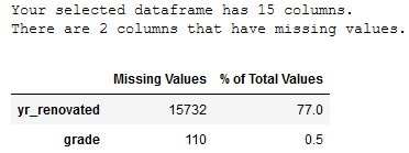
Due to the high number of missing values (>75%) the column yr_renovated should not be considered in the further analysis.
'''
Delete the column yr_renovated
'''

df_without_outliers = df_without_outliers.drop(['yr_renovated'], axis=1)
df_without_outliers.head()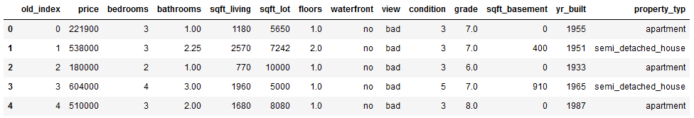
Due to the low number of Missing Values within the grade column, this column will not be deleted as valuable information could be lost. The missing values should be filled with the mean value of the column instead.
'''
Impute missing values for column grade
'''

df_without_outliers['grade'] = df_without_outliers['grade'].fillna(df_without_outliers['grade'].mean())
Check if all missing values are removed or replaced.
missing_values_table(df_without_outliers)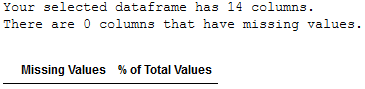
According to our best practice approach we will assign a new name to the data set.
df_without_MV = df_without_outliers4.1.3 Handling Categorical Variables
Now we are going to handle the categorical variables.
obj_col = ['object']
object_columns = list(df_without_MV.select_dtypes(include=obj_col).columns)
house_prices_categorical = df_without_MV[object_columns]

print()
print('There are ' + str(house_prices_categorical.shape[1]) + ' categorical columns within dataframe:')

house_prices_categorical.head()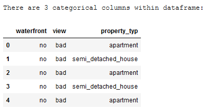
print('Values of the variable waterfront:')
print()
print(df_without_MV['waterfront'].value_counts())

print('--------------------------------------------')

print('Values of the variable view:')
print()
print(df_without_MV['view'].value_counts())

print('--------------------------------------------')

print('Values of the variable property_typ:')
print()
print(df_without_MV['property_typ'].value_counts())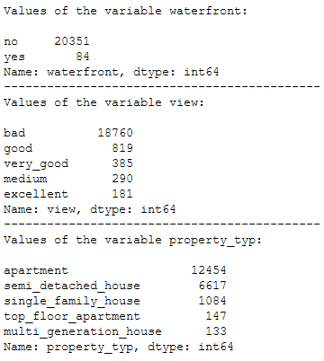
Based on the output shown above, the following scale level can be determined for the three categorical variables:
- waterfront: binary
- view: ordinal
- property_typ: nominal
The variables will be coded accordingly in the following.
'''
In the following the column waterfront is coded.
Then the newly generated values are inserted into the original dataframe
and the old column will be deleted.
'''

encoder_waterfront = LabelBinarizer()

# Application of the LabelBinarizer
waterfront_encoded = encoder_waterfront.fit_transform(df_without_MV.waterfront.values.reshape(-1,1))

# Insertion of the coded values into the original data set
df_without_MV['waterfront_encoded'] = waterfront_encoded

# Delete the original column to avoid duplication
df_without_MV = df_without_MV.drop(['waterfront'], axis=1)

# Getting the exact coding and show new dataframe
print(encoder_waterfront.classes_)
print('Codierung: no=0, yes=1')
print('-----------------------------')
print()
print('New Data Frame:')
df_without_MV.head()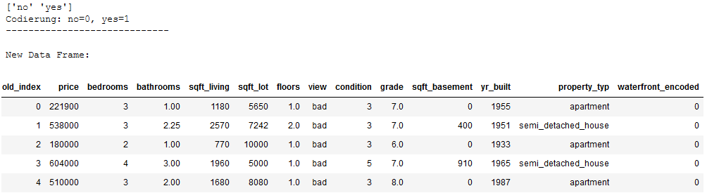
'''
In the following the column view is coded.
Then the newly generated values are inserted into the original dataframe
and the old column will be deleted.
'''

# Create a dictionary how the observations should be coded
view_dict = {'bad' : 0,
             'medium' : 1,
             'good' : 2,
             'very_good' : 3,
             'excellent' : 4}

# Map the dictionary on the column view and store the results in a new column
df_without_MV['view_encoded'] = df_without_MV.view.map(view_dict)

# Delete the original column to avoid duplication
df_without_MV = df_without_MV.drop(['view'], axis=1)


print('New Data Frame:')
df_without_MV.head()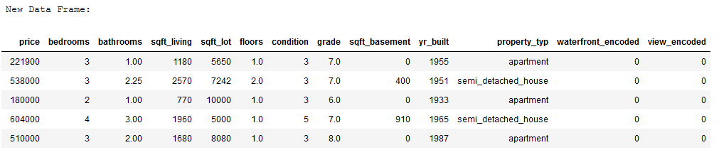
'''
In the following the column property_typ is coded.
Then the newly generated values are inserted into the original dataframe
and the old column will be deleted.
'''

encoder_property_typ = OneHotEncoder()

# Application of the OneHotEncoder
OHE = encoder_property_typ.fit_transform(df_without_MV.property_typ.values.reshape(-1,1)).toarray()

# Conversion of the newly generated data to a dataframe
df_OHE = pd.DataFrame(OHE, columns = ["property_typ_" + str(encoder_property_typ.categories_[0][i])
                                     for i in range(len(encoder_property_typ.categories_[0]))])


# Insertion of the coded values into the original data set
df_without_MV = pd.concat([df_without_MV, df_OHE], axis=1)


# Delete the original column to avoid duplication
df_without_MV = df_without_MV.drop(['property_typ'], axis=1)


print('New Data Frame:')
df_without_MV.head()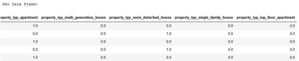
Now that the record is clean we can rename it accordingly. It is also recommended to save the clean data set at this point.
final_df_house_prices = df_without_MV

final_df_house_prices.to_csv('dataframes/final_df_house_prices.csv', index=False)
4.2 Research Question 1
The first research question is:
Is there a difference in the characteristics of the properties, if they are located on a waterfront?
print('Absolute distribution: ')
print()
print(final_df_house_prices['waterfront_encoded'].value_counts())

print('-------------------------------------------------------')

print('Percentage distribution: ')
print()
print(pd.DataFrame({'Percentage': final_df_house_prices.groupby(('waterfront_encoded')).size() / len(final_df_house_prices)}))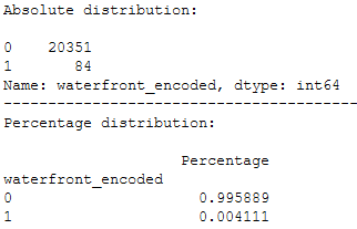
final_df_house_prices.groupby(('waterfront_encoded')).mean()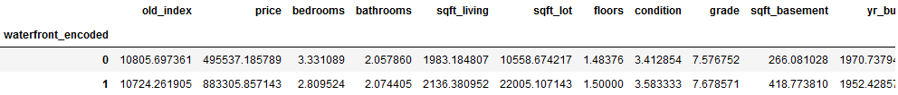
Answer the first research question:
The average price for waterfront properties is almost twice as high as for other properties.
On the other hand, the difference in the average plot size is not so great.
If one regards the year of construction of the real estates then one can state that the houses at a waterfront are average 18 years older.
4.3 Research Question 2
The second research question is:
What clusters are there in terms of real estate?
# Here we drop the column old_index because we do not want to cluster these features

house_prices_cluster = final_df_house_prices.drop(['old_index'], axis=1)
house_prices_cluster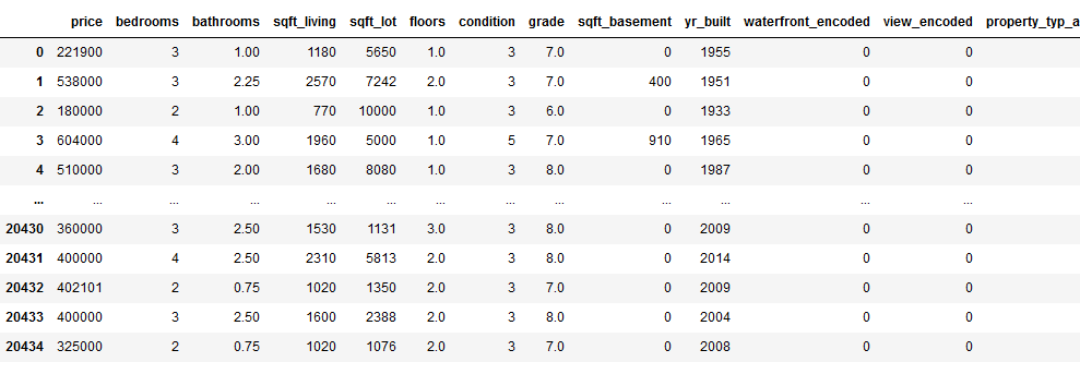
Let’s have another look at the distribution of the variable ‘house prices’. This time not with a box plot but with a histogram.
plt.hist(house_prices_cluster['price'], bins='auto')
plt.title("Histogram for house prices")
plt.xlim(xmin=0, xmax = 1200000)
plt.show()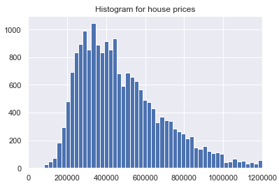
mms = MinMaxScaler()
mms.fit(house_prices_cluster)
data_transformed = mms.transform(house_prices_cluster)
Sum_of_squared_distances = []
K = range(1,15)
for k in K:
km = KMeans(n_clusters=k)
km = km.fit(data_transformed)
Sum_of_squared_distances.append(km.inertia_)plt.plot(K, Sum_of_squared_distances, 'bx-')
plt.xlabel('k')
plt.ylabel('Sum_of_squared_distances')
plt.title('Elbow Method For Optimal k')
plt.show()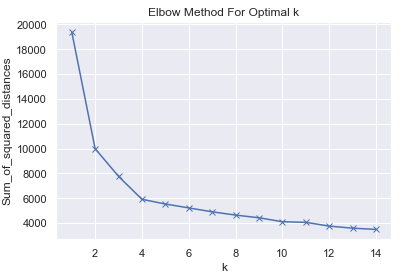
km = KMeans(n_clusters=4, random_state=1)
km.fit(house_prices_cluster)
predict=km.predict(house_prices_cluster)
house_prices_cluster['clusters'] = pd.Series(predict, index=house_prices_cluster.index)df_sub = house_prices_cluster[['sqft_living', 'price']].values
plt.scatter(df_sub[predict==0, 0], df_sub[predict==0, 1], s=100, c='red', label ='Cluster 1')
plt.scatter(df_sub[predict==1, 0], df_sub[predict==1, 1], s=100, c='blue', label ='Cluster 2')
plt.scatter(df_sub[predict==2, 0], df_sub[predict==2, 1], s=100, c='green', label ='Cluster 3')
plt.scatter(df_sub[predict==3, 0], df_sub[predict==3, 1], s=100, c='cyan', label ='Cluster 4')
plt.title('Cluster of Houses')
plt.xlim((0, 5000))
plt.ylim((0,2000000))
plt.xlabel('sqft_living \n\n Cluster1(Red), Cluster2 (Blue), Cluster3(Green), Cluster4(Cyan)')
plt.ylabel('Price')
plt.show()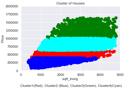
Answer the second research question:
Within the data set 4 clusters could be identified. We can see in the graphic above that the target buyer groups of the houses can be clearly defined. In this case, targeted customer segmentation and personalized recommendations from a marketing point of view would now be an option.
4.4 Research Question 3
The third research question is:
Does the number of square meters have a significant influence on the price of the property?
To answer the research question we filter the data set for the variable price and sqft_living.
HousePrices_SimplReg = final_df_house_prices[['price', 'sqft_living']]
HousePrices_SimplReg.head()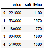
x = HousePrices_SimplReg['sqft_living']
y = HousePrices_SimplReg['price']

plt.scatter(x, y)
plt.title('Scatter plot: sqft_living vs. price')
plt.xlabel('sqft_living')
plt.ylabel('price')
plt.show()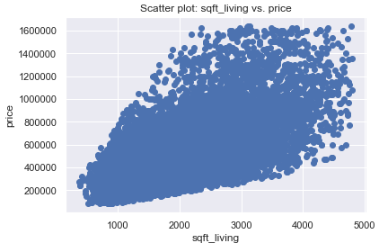
model1 = smf.ols(formula='price~sqft_living', data=HousePrices_SimplReg).fit()

model1.summary()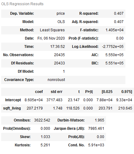
Answer the third research question:
As we can see from the p value, it is highly significant. It can therefore be assumed that the number of square meters is a significant predictor of the price of a property.
5 Development of a Machine Learning Model End to End Process
Now that the descriptive part has been completed and the research questions posed at the beginning have been answered, we now come to the second main part of this publication.
The training of a machine learning model for predicting house prices.
A golden rule in Data Science
For the development of a machine learning algorithm it is imperative that all pre-processing steps are applied to the training part only! Anything else would negatively affect the later performance of the algorithm. Outliers are the only exceptions to this rule. Here it always depends on the respective data set and its size.
Often I have found that this rule is not followed. This has been one of the motivations for me to describe a complete end-to-end process for the development of machine learning models in this post.
The further procedure follows the Best Practice approach for ML Model Development. I have listed this approach at the end of this publication (chapter 7). You can also download these instructions here: “DS Best Practice Guidlines for ML Model Development”. It allows you to track the naming convention used and to see when which models, data sets or stored metrics are saved.
5.1 Data pre-processing
Due to the fact that we have to approach the pre-processing steps a bit differently to create an ML algorithm, we reload the original data set.
house_prices = pd.read_csv("house_prices_dataframe.csv")
house_prices.head()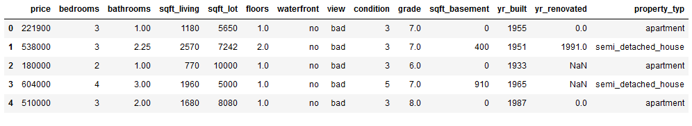
5.1.1 Train Test Split
Here we are going to split the data into a training part (80%) and a test part (20%).
x = house_prices.drop(['price'], axis=1)
y = house_prices['price']

trainX, testX, trainY, testY = train_test_split(x, y, test_size = 0.2)
At this point it is recommended to reset the index of the 4 created ‘records’ and to delete the old index (which is automatically generated as new column).
trainX = trainX.reset_index().drop(['index'], axis=1)
testX = testX.reset_index().drop(['index'], axis=1)
trainY = trainY.reset_index().drop(['index'], axis=1)
testY = testY.reset_index().drop(['index'], axis=1)
5.1.2 Removal of Outlier
# Define the outlier-detect function
def outliers_z_score(df):
    threshold = 3

    mean = np.mean(df)
    std = np.std(df)
    z_scores = [(y - mean) / std for y in df]
    return np.where(np.abs(z_scores) > threshold)

# For the further proceeding we just need numerical colunns
my_list = ['int16', 'int32', 'int64', 'float16', 'float32', 'float64']
num_columns = list(trainX.select_dtypes(include=my_list).columns)
numerical_columns = trainX[num_columns]

# Now we are going to apply our outlier-function to all numerical columns
outlier_list = numerical_columns.apply(lambda x: outliers_z_score(x))
outlier_list

# Store the results within a dataframe
df_of_outlier = outlier_list.iloc[0]
df_of_outlier = pd.DataFrame(df_of_outlier)
df_of_outlier.columns = ['Rows_to_exclude']


# Convert all values from column Rows_to_exclude to a numpy array
outlier_list_final = df_of_outlier['Rows_to_exclude'].to_numpy()

# Concatenate a whole sequence of arrays
outlier_list_final = np.concatenate( outlier_list_final, axis=0 )

# Drop dubplicate values
outlier_list_final_unique = set(outlier_list_final)

# Create a new dataframe without the identified outlier
filter_rows_to_exclude = trainX.index.isin(outlier_list_final_unique)
trainX_wo_outlier = trainX[~filter_rows_to_exclude]

# Reset the index again
trainX_wo_outlier = trainX_wo_outlier.reset_index().drop(['index'], axis=1)
print('Length of original dataframe: ' + str(len(trainX)))
print('Length of new dataframe without outliers: ' + str(len(trainX_wo_outlier)))
print('----------------------------------------------------------------------------------------------------')
print('Difference between new and old dataframe: ' + str(len(trainX) - len(trainX_wo_outlier)))
print('----------------------------------------------------------------------------------------------------')
print('Length of unique outlier list: ' + str(len(outlier_list_final_unique)))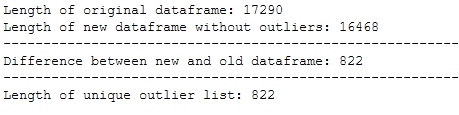
Of course it is now also necessary to remove the corresponding Y values of the outlier.
filter_rows_to_exclude = trainY.index.isin(outlier_list_final_unique)
trainY_wo_outlier = trainY[~filter_rows_to_exclude]

trainY_wo_outlier = trainY_wo_outlier.reset_index().drop(['index'], axis=1)
print('Length of original dataframe: ' + str(len(trainY)))
print('Length of new dataframe without outliers: ' + str(len(trainY_wo_outlier)))
print('----------------------------------------------------------------------------------------------------')
print('Difference between new and old dataframe: ' + str(len(trainY) - len(trainY_wo_outlier)))
print('----------------------------------------------------------------------------------------------------')
print('Length of unique outlier list: ' + str(len(outlier_list_final_unique)))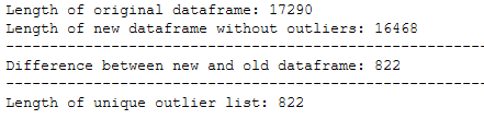
5.1.3 Missing Values
def missing_values_table(df):
        # Total missing values
        mis_val = df.isnull().sum()

        # Percentage of missing values
        mis_val_percent = 100 * df.isnull().sum() / len(df)

        # Make a table with the results
        mis_val_table = pd.concat([mis_val, mis_val_percent], axis=1)

        # Rename the columns
        mis_val_table_ren_columns = mis_val_table.rename(
        columns = {0 : 'Missing Values', 1 : '% of Total Values'})

        # Sort the table by percentage of missing descending
        mis_val_table_ren_columns = mis_val_table_ren_columns[
            mis_val_table_ren_columns.iloc[:,1] != 0].sort_values(
        '% of Total Values', ascending=False).round(1)

        # Print some summary information
        print ("Your selected dataframe has " + str(df.shape[1]) + " columns.\n"
            "There are " + str(mis_val_table_ren_columns.shape[0]) +
              " columns that have missing values.")

        # Return the dataframe with missing information
        return mis_val_table_ren_columns


missing_values_table(trainX_wo_outlier)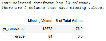
# Deletion of the column yr_renovated because too many missing values.

trainX_wo_outlier = trainX_wo_outlier.drop(['yr_renovated'], axis=1)
# Impute missing values for column grade with mean values of this columns
trainX_wo_outlier['grade'] = trainX_wo_outlier['grade'].fillna(trainX_wo_outlier['grade'].mean())# Check if all missing values are removed or replaced.
missing_values_table(trainX_wo_outlier)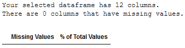
Of course it can happen that the data we get later to the predicte also has some missing values. To be able to fill these values in a meaningful way it is advisable to save the corresponding metrics from the original trainings part (for example the average value of a column).
mean_grade = trainX_wo_outlier['grade'].mean()
mean_condition = trainX_wo_outlier['condition'].mean()
mean_sqft_living = trainX_wo_outlier['sqft_living'].mean()
mean_sqft_lot = trainX_wo_outlier['sqft_lot'].mean()


pk.dump(mean_grade, open('metrics_MV/mean_grade.pkl', 'wb'))
pk.dump(mean_condition, open('metrics_MV/mean_condition.pkl', 'wb'))
pk.dump(mean_sqft_living, open('metrics_MV/mean_sqft_living.pkl', 'wb'))
pk.dump(mean_sqft_lot, open('metrics_MV/mean_sqft_lot.pkl', 'wb'))


print('Mean of column grade: ' + str(mean_grade))
print('Mean of column condition: ' + str(mean_condition))
print('Mean of column sqft_living: ' + str(mean_sqft_living))
print('Mean of column sqft_lot: ' + str(mean_sqft_lot))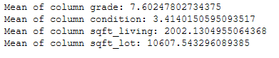
To comply with the best practice approach, we assign a new name (trainX_wo_MV) to the data set (trainX_wo_outlier).
trainX_wo_MV = trainX_wo_outlier5.1.4 Categorical Variables
obj_col = ['object']
object_columns = list(trainX_wo_MV.select_dtypes(include=obj_col).columns)
trainX_categorical = trainX_wo_MV[object_columns]

print()
print('There are ' + str(trainX_categorical.shape[1]) + ' categorical columns within dataframe(trainX).')
As we already know from the descriptive part, the three categorical variables are scaled as follows:
- waterfront: binary
- view: ordinal
- property_typ: nominal
The variables will be coded accordingly in the following.
'''
In the following the column waterfront is coded.
Then the newly generated values are inserted into the original dataframe
and the old column will be deleted.
'''

encoder_waterfront = LabelBinarizer()

# Application of the LabelBinarizer
waterfront_encoded = encoder_waterfront.fit_transform(trainX_wo_MV.waterfront.values.reshape(-1,1))

# Insertion of the coded values into the original data set
trainX_wo_MV['waterfront_encoded'] = waterfront_encoded

# Delete the original column to avoid duplication
trainX_wo_MV = trainX_wo_MV.drop(['waterfront'], axis=1)
'''
In the following the column view is coded.
Instead of the OrdinalEncoder from scikit learn I prefer to use a dictionary,
because I can specify the exact ordinal order here.
I also design an inverse dictionary to encode the data back later if needed.
Then the newly generated values are inserted into the original dataframe
and the old column will be deleted.
'''
# Create a dictionary how the observations should be coded
view_dict = {'bad' : 0,
'medium' : 1,
'good' : 2,
'very_good' : 3,
'excellent' : 4}
view_dict_inverse = {0 : 'bad',
1 : 'medium',
2 : 'good',
3 : 'very_good',
4 : 'excellent'}
# Map the dictionary on the column view and store the results in a new column
trainX_wo_MV['view_encoded'] = trainX_wo_MV.view.map(view_dict)
# Delete the original column to avoid duplication
trainX_wo_MV = trainX_wo_MV.drop(['view'], axis=1)'''
In the following the column property_typ is coded.
Then the newly generated values are inserted into the original dataframe
and the old column will be deleted.
'''
encoder_property_typ = OneHotEncoder()
# Application of the OneHotEncoder
OHE = encoder_property_typ.fit_transform(trainX_wo_MV.property_typ.values.reshape(-1,1)).toarray()
# Conversion of the newly generated data to a dataframe
df_OHE = pd.DataFrame(OHE, columns = ["property_typ_" + str(encoder_property_typ.categories_[0][i])
for i in range(len(encoder_property_typ.categories_[0]))])
# Insertion of the coded values into the original data set
trainX_wo_MV = pd.concat([trainX_wo_MV, df_OHE], axis=1)
# Delete the original column to avoid duplication
trainX_wo_MV = trainX_wo_MV.drop(['property_typ'], axis=1)An often forgotten step but a very important necessity is to store the fitted encoders or used dictionaries separately to be able to use them after deployment for predictions on new data.
pk.dump(encoder_waterfront, open('encoder/encoder_waterfront.pkl', 'wb'))
pk.dump(view_dict, open('encoder/view_dict.pkl', 'wb'))
pk.dump(view_dict_inverse, open('encoder/view_dict_inverse.pkl', 'wb'))
pk.dump(encoder_property_typ, open('encoder/encoder_property_typ.pkl', 'wb'))


print('Classes of encoder_waterfront :')
print(encoder_waterfront.classes_)
print('Codierung: no=0, yes=1')
print()
print('------------------------------------------------')
print()
print('Assignments by the dictionary for view :')
print(view_dict)
print()
print('------------------------------------------------')
print()
print('Assignments by the inverse dictionary for view :')
print(view_dict_inverse)
print()
print('------------------------------------------------')
print()
print('Categories of encoder_property_typ :')
print(encoder_property_typ.categories_)
print()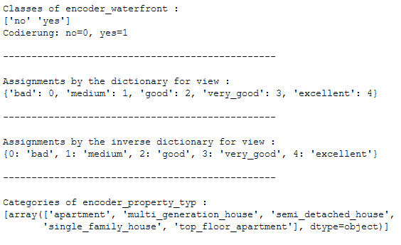
Once again we keep to the naming convention and adhere to the requirement to save the currently created data set.
trainX_encoded = trainX_wo_MV

trainX_encoded.to_csv('dataframes/trainX_encoded.csv', index=False)
5.1.5 Scaling
Another important pre-processing step is the scaling of the data. We will apply the standard scaler to the trainX_wo_outlier data set and save the fitted scaler for later transformations.
col_names = trainX_encoded.columns
features = trainX_encoded[col_names]

scaler = StandardScaler().fit(features.values)
features = scaler.transform(features.values)

trainX_scaled = pd.DataFrame(features, columns = col_names)
trainX_scaled.head()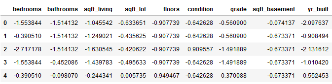
As announced also this scaler is stored for later predictions.
pk.dump(scaler, open('scaler/StandardScaler.pkl', 'wb'))5.2 Filter Methods
5.2.1 Dealing with Highly Correlated Features
Now that all variables are numeric it is easy to create a correlation plot. This gives a first insight into which variables seem to correlate highly.
plt.figure(figsize=(8,6))
cor = trainX_scaled.corr()
sns.heatmap(cor, annot=True, cmap=plt.cm.Reds)
plt.show()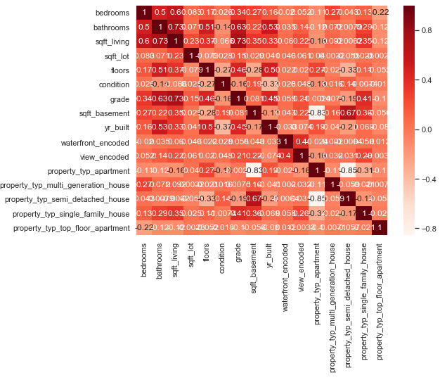
With the following commands I check if highly correlated variables exist. If so, we would have to exclude them, since this is a prerequisite for regression analysis. As we can see, this is not the case here.
correlated_features = set()
correlation_matrix = trainX_scaled.corr()

threshold = 0.90

for i in range(len(correlation_matrix .columns)):
    for j in range(i):
        if abs(correlation_matrix.iloc[i, j]) > threshold:
            colname = correlation_matrix.columns[i]
            correlated_features.add(colname)


len(correlated_features)
5.2.2 Dealing with Constant Features
It is as important as the highly correlated variables to check whether constant features or quasi constant features exist. Also this is not the case here. No further variables must be excluded.
constant_filter = VarianceThreshold(threshold=0)
constant_filter.fit(trainX_scaled)


constant_columns = [column for column in trainX_scaled.columns
                    if column not in trainX_scaled.columns[constant_filter.get_support()]]


qconstant_filter = VarianceThreshold(threshold=0.01)
qconstant_filter.fit(trainX_scaled)


qconstant_columns = [column for column in trainX_scaled.columns
                    if column not in trainX_scaled.columns[qconstant_filter.get_support()]]


print('Number of constant features: ' + str(len(constant_columns)))
print('Number of constant features: ' + str(len(qconstant_columns)))
5.2.3 Dealing with Duplicate Features
Finally we check if duplicated features exist. This is also not the case.
trainX_scaled_T = trainX_scaled.T

print('Number of duplicate features: ' + str(trainX_scaled_T.duplicated().sum()))
Due to the fact that we did not have to exclude any other features, the following two training data sets are the ones we want to continue working with:
trainX_final = trainX_scaled
trainY_final = trainY_wo_outlier
Furthermore, the respective final data sets are also to be stored at this point.
trainX_final.to_csv('dataframes/trainX_final.csv', index=False)
trainY_final.to_csv('dataframes/trainY_final.csv', index=False)
5.3 ML-Model Development
5.3.1 Training
Subsequently, the regression model is created, trained and its R² value is calculated.
It is also stored for test purposes and validation.
lm = LinearRegression()
lm.fit(trainX_final, trainY_final)

print('R² Score of fitted lm-model: ' + str(lm.score(trainX_final, trainY_final)))

pk.dump(lm, open('model/lm_model.pkl', 'wb'))
5.3.2 Testing
You can consider the test data set as a completely independent new data set on which to make predictions. This means that we have to do all pre-processing steps (coding, scaling, removing columns etc.) again.
This is a step that is a bit more complex and is avoided by many developers by first pre-processing the data and then doing a train-test split, but it is the closest to the truth.
Now we will also need most of the previously saved files (saved mean values, scalers etc.).
5.3.2.1 Missing Values
We know from the previous analysis that we excluded the column yr_renovated because of the high number of missing values.
We also know that the column grade also contains missing values and we should fill it with the stored mean_grade.
We will do this in the following.
Outliers are no longer identified and excluded, as it is now the test data set.
# Deletion of the column yr_renovated because too many missing values.
testX = testX.drop(['yr_renovated'], axis=1)

# Impute missing values for column grade with with the average values of this column from the training data set.
mean_grade_reload = pk.load(open("metrics_MV/mean_grade.pkl",'rb'))
testX['grade'] = testX['grade'].fillna(mean_grade_reload)

# Rename testX according best practice guideline
testX_wo_MV = testX
5.3.2.2 Categorical Variables
We also know from the past which variables are categorical and how they must be coded accordingly. This time we only use the saved encoders and the saved dictionaries.
Watch out!
With the loaded encoder only the transform function will be used from now on. In no case the fit_transform function is used, because otherwise new values would be generated.
# Load the necessary encoder/dic
encoder_waterfront_reload = pk.load(open("encoder/encoder_waterfront.pkl",'rb'))
view_dict_reload = pk.load(open("encoder/view_dict.pkl",'rb'))
encoder_property_typ_reload = pk.load(open("encoder/encoder_property_typ.pkl",'rb'))


# Application of the reload LabelBinarizer
waterfront_encoded = encoder_waterfront_reload.transform(testX_wo_MV.waterfront.values.reshape(-1,1))
# Insertion of the coded values into the original data set
testX_wo_MV['waterfront_encoded'] = waterfront_encoded
# Delete the original column to avoid duplication
testX_wo_MV = testX_wo_MV.drop(['waterfront'], axis=1)


# Map the reload dictionary on the column view and store the results in a new column
testX_wo_MV['view_encoded'] = testX_wo_MV.view.map(view_dict_reload)
# Delete the original column to avoid duplication
testX_wo_MV = testX_wo_MV.drop(['view'], axis=1)


# Application of the reload OneHotEncoder
OHE = encoder_property_typ_reload.transform(testX_wo_MV.property_typ.values.reshape(-1,1)).toarray()
# Conversion of the newly generated data to a dataframe
df_OHE = pd.DataFrame(OHE, columns = ["property_typ_" + str(encoder_property_typ_reload.categories_[0][i])
                                      for i in range(len(encoder_property_typ_reload.categories_[0]))])
# Insertion of the coded values into the original data set
testX_wo_MV = pd.concat([testX_wo_MV, df_OHE], axis=1)
# Delete the original column to avoid duplication
testX_wo_MV = testX_wo_MV.drop(['property_typ'], axis=1)
At this point we will rename the data set accordingly and also save it separately.
# Rename testX_wo_MV according best practice guideline
testX_encoded = testX_wo_MV


testX_encoded.to_csv('dataframes/testX_encoded.csv', index=False)
5.3.2.3 Scaling
Like the coding, the testX data must be scaled using the same metrics calculated from the training data.
# Load the necessary scaler
scaler_reload = pk.load(open("scaler/StandardScaler.pkl",'rb'))


col_names = testX_encoded.columns
features = testX_encoded[col_names]

features = scaler_reload.transform(features.values)
testX_scaled = pd.DataFrame(features, columns = col_names)
Since we did not find any variables in the filter methods, we have to exclude them, this step is skipped in the test data.
However, we still rename the data sets accordingly and store them separately.
testX_final = testX_scaled
testY_final = testY

testX_final.to_csv('dataframes/testX_final.csv', index=False)
testY_final.to_csv('dataframes/testY_final.csv', index=False)
5.3.2.4 Test the ML-Model
Now it is time to test the saved lm model. For this we reload it and predicted the house prices. In the following an evaluation will take place.
# Reload the model
lm_reload = pk.load(open("model/lm_model.pkl",'rb'))

# Predict values for test dataset
y_pred = lm_reload.predict(testX_final)

# Create a dataset with actual and predicted values
y_pred_df = pd.DataFrame(y_pred)
y_pred_df.columns = ['values_predicted']
actual_vs_predicted = pd.concat([testY_final, y_pred_df], axis=1)

# Visualize the results
df1 = actual_vs_predicted.head(30)
df1.plot(kind='bar',figsize=(10,6))
plt.grid(which='major', linestyle='-', linewidth='0.5', color='green')
plt.grid(which='minor', linestyle=':', linewidth='0.5', color='black')
plt.show()

# Print some validation metrics
print('Mean Absolute Error:', metrics.mean_absolute_error(testY_final, y_pred))
print('Mean Squared Error:', metrics.mean_squared_error(testY_final, y_pred))
print('Root Mean Squared Error:', np.sqrt(metrics.mean_squared_error(testY_final, y_pred)))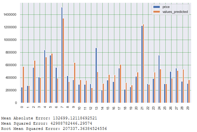
5.4 Feature Selection
Now that we have successfully developed a ml model, we try to improve it again by selecting only the most important features (via RFE).
5.4.1 Recursive Feature Elimination
lr = LinearRegression()

rfe = RFE(lr, n_features_to_select=10)
rfe.fit(trainX_final, trainY_final)
Columns = trainX_final.columns
RFE_support = rfe.support_
RFE_ranking = rfe.ranking_
dataset = pd.DataFrame({'Columns': Columns, 'RFE_support': RFE_support, 'RFE_ranking': RFE_ranking}, columns=['Columns', 'RFE_support', 'RFE_ranking'])
dataset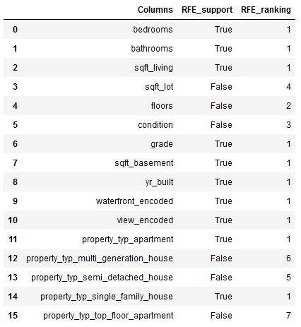
df = dataset[(dataset["RFE_support"] == True) & (dataset["RFE_ranking"] == 1)]
filtered_features = df['Columns']
filtered_features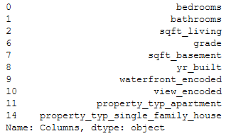
pk.dump(filtered_features, open('feature_selection_RFE/filtered_features_RFE.pkl', 'wb'))5.4.2 Training
Due to the fact that we will now consider a new number of variables, we have to reapply and save the scaler. If we don’t do that, we will have problems later on to transform the data back to make it readable.
The scaler remembers the number of columns and the order of the columns. For example, you can not scale 5 columns and only try to transform 4 back. If you take this into account in the preparation, you often save yourself additional work later.
For this step we reload the anticipatory stored data set trainX_encoded, apply the filter from feature selection RFE (filtered_features_RFE) to it and rescale it (and of course save the new scaler again).
trainX_encoded_reload = pd.read_csv("dataframes/trainX_encoded.csv")
trainX_encoded_reload.head()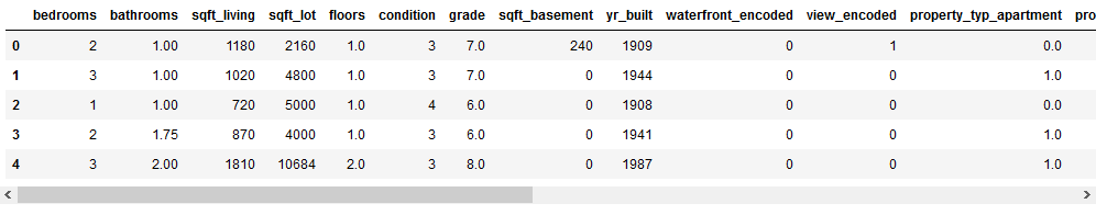
5.4.2.1 Column Selection according RFE
As announced shortly before, we load the filter from RFE and apply it.
filtered_features_RFE_reload = pk.load(open("feature_selection_RFE/filtered_features_RFE.pkl",'rb'))

trainX_FS = trainX_encoded_reload[filtered_features_RFE_reload]
5.4.2.2 New Scaling
col_names = trainX_FS.columns
features = trainX_FS[col_names]

scaler = StandardScaler().fit(features.values)
features = scaler.transform(features.values)

trainX_FS_scaled = pd.DataFrame(features, columns = col_names)


pk.dump(scaler, open('scaler/StandardScaler2.pkl', 'wb'))
As a last step, we rename the data sets for x and y again and save them.
trainX_final2 = trainX_FS_scaled
trainY_final2 = trainY_final

trainX_final2.to_csv('dataframes/trainX_final2.csv', index=False)
trainY_final2.to_csv('dataframes/trainY_final2.csv', index=False)
5.4.2.3 Fit the new ML-Model
Here a new training starts due to the data situation after feature selection.
lm2 = LinearRegression()
lm2.fit(trainX_final2, trainY_final2)

print('R² Score of fitted lm2-model: ' + str(lm2.score(trainX_final2, trainY_final2)))

pk.dump(lm2, open('model/lm2_model.pkl', 'wb'))
5.4.3 Testing
As in the training part after RFE we have to select the column via the RFE filter and rescale it.
testX_encoded_reload = pd.read_csv("dataframes/testX_encoded.csv")
testX_encoded_reload.head()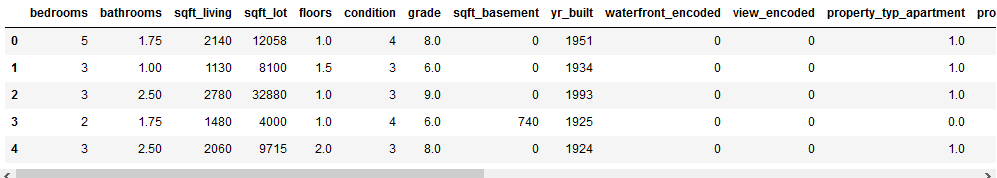
5.4.3.1 Column Selection according RFE
As announced shortly before, we load the filter from RFE and apply it.
filtered_features_RFE_reload = pk.load(open("feature_selection_RFE/filtered_features_RFE.pkl",'rb'))

testX_FS = testX_encoded_reload[filtered_features_RFE_reload]
5.4.3.2 New Scaling
Like the coding, the testX data must be scaled using the same metrics calculated from the training data.
# Load the necessary scaler
scaler2_reload = pk.load(open("scaler/StandardScaler2.pkl",'rb'))


col_names = testX_FS.columns
features = testX_FS[col_names]

features = scaler2_reload.transform(features.values)

testX_FS_scaled = pd.DataFrame(features, columns = col_names)
testX_final2 = testX_FS_scaled
testY_final2 = testY_final
testX_final2.to_csv('dataframes/testX_final.csv', index=False)
testY_final2.to_csv('dataframes/testY_final.csv', index=False)5.4.3.3 Test the new ML-Model
Now we will test the newly created lm model (based on feature selection).
# Reload the model
lm2_reload = pk.load(open("model/lm2_model.pkl",'rb'))

# Predict values for test dataset
y_pred = lm2_reload.predict(testX_final2)


# Create a dataset with actual and predicted values
y_pred_df = pd.DataFrame(y_pred)
y_pred_df.columns = ['values_predicted']
actual_vs_predicted = pd.concat([testY_final2, y_pred_df], axis=1)

# Visualize the results
df1 = actual_vs_predicted.head(30)
df1.plot(kind='bar',figsize=(10,6))
plt.grid(which='major', linestyle='-', linewidth='0.5', color='green')
plt.grid(which='minor', linestyle=':', linewidth='0.5', color='black')
plt.show()

# Print some validation metrics
print('Mean Absolute Error:', metrics.mean_absolute_error(testY_final2, y_pred))
print('Mean Squared Error:', metrics.mean_squared_error(testY_final2, y_pred))
print('Root Mean Squared Error:', np.sqrt(metrics.mean_squared_error(testY_final2, y_pred)))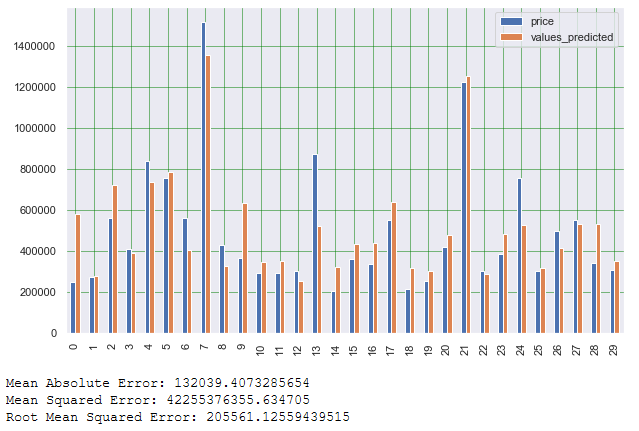
As we can see from the Mean Absolut Error (MAE), the lm2 model has improved slightly compared to the first model. The same applies to the Mean Squared Error as well as Root Mean Squared Error.
At this point we now have completely prepared training and test data on which the performance of various algorithms can be tested.My recommendation at this point is to always start with ‘simple’ algorithms (like the linear regression model) and then to use more and more complex algorithms (random forest, ensemble methods up to neural networks).
Furthermore you can use hyperparameter tuning (with grid-search) to improve the performance.
As we have seen, the data preprocessing has taken the most time. Now comes the best part, the magic with different machnie learning models.
5.5 Out-Of-The-Box-Data
So far we have prepared the data accordingly, developed a machine learning model and improved it using feature selection. Now we can test it again with completely new data.
This is, for example, the description of the property I am currently living in. I am curious to see what value is predicted for my property.
my_property = pd.DataFrame({
                   'bedrooms': [3],
                   'bathrooms': [2],
                   'sqft_living': [180],
                   'sqft_lot': [1300],
                   'floors': [2],
                   'waterfront': ['yes'],
                   'view': ['good'],
                   'condition': [np.NaN],
                   'grade': [4],
                   'sqft_basement': [300],
                   'yr_built': [1950],
                   'yr_renovated': [2001],
                   'property_typ': ['apartment']})
my_property
5.5.1 Missing Values
First I replace all missing values again. This time the columned condition is filled with NaN and will be replaced by me.
# Deletion of the column yr_renovated because too many missing values.
my_property = my_property.drop(['yr_renovated'], axis=1)

# Impute missing values for column condition with with the average values of this column from the training data set.
mean_condition_reload = pk.load(open("metrics_MV/mean_condition.pkl",'rb'))
my_property['condition'] = my_property['condition'].fillna(mean_condition_reload)

my_property_wo_MV = my_property
5.5.2 Cat Var
As known, the coding of the categorical variables is also carried out.
# Load the necessary encoder/dic
encoder_waterfront_reload = pk.load(open("encoder/encoder_waterfront.pkl",'rb'))
view_dict_reload = pk.load(open("encoder/view_dict.pkl",'rb'))
encoder_property_typ_reload = pk.load(open("encoder/encoder_property_typ.pkl",'rb'))


# Application of the reload LabelBinarizer
waterfront_encoded = encoder_waterfront_reload.transform(my_property_wo_MV.waterfront.values.reshape(-1,1))
# Insertion of the coded values into the original data set
my_property_wo_MV['waterfront_encoded'] = waterfront_encoded
# Delete the original column to avoid duplication
my_property_wo_MV = my_property_wo_MV.drop(['waterfront'], axis=1)


# Map the reload dictionary on the column view and store the results in a new column
my_property_wo_MV['view_encoded'] = my_property_wo_MV.view.map(view_dict_reload)
# Delete the original column to avoid duplication
my_property_wo_MV = my_property_wo_MV.drop(['view'], axis=1)


# Application of the reload OneHotEncoder
OHE = encoder_property_typ_reload.transform(my_property_wo_MV.property_typ.values.reshape(-1,1)).toarray()
# Conversion of the newly generated data to a dataframe
df_OHE = pd.DataFrame(OHE, columns = ["property_typ_" + str(encoder_property_typ_reload.categories_[0][i])
                                      for i in range(len(encoder_property_typ_reload.categories_[0]))])
# Insertion of the coded values into the original data set
my_property_wo_MV = pd.concat([my_property_wo_MV, df_OHE], axis=1)
# Delete the original column to avoid duplication
my_property_wo_MV = my_property_wo_MV.drop(['property_typ'], axis=1)


my_property_encoded = my_property_wo_MV
5.5.3 Column Selection according RFE
Next we are going to do the column selection according RFE
filtered_features_RFE_reload = pk.load(open("feature_selection_RFE/filtered_features_RFE.pkl",'rb'))

my_property_encoded = my_property_encoded[filtered_features_RFE_reload]


my_property_FS = my_property_encoded
5.5.4 Scaling
Last but not least feature scaling.
# Load the necessary scaler
scaler2_reload = pk.load(open("scaler/StandardScaler2.pkl",'rb'))


col_names = my_property_FS.columns
features = my_property_FS[col_names]

features = scaler2_reload.transform(features.values)

my_property_FS_scaled = pd.DataFrame(features, columns = col_names)
5.5.5 Prediction of new Values
Now I will use the final created model to predict the price for my property.
# Reload the model
lm2_reload = pk.load(open("model/lm2_model.pkl",'rb'))

# Predict values for my dataset
y_pred = lm2_reload.predict(my_property_FS_scaled)

print('The predicted price for my property is: ' + str(y_pred))
6 Conclusion
In this publication I have shown how to prepare data in a meaningful way to extract valuable insights (answers to research questions). I also covered all steps of developing and evaluating a machine learning model.
Here is an overview how I proceeded with the development of a machine learning model:
Data pre-processing
- Outliers
- Missing Values
- Feature Encoding
- Feature Scaling
Filter Methods
- Highly correlated features
- Constant features
- Duplicate features
Model Traing & Testing
- Simple Models (eg. linear Regression)
- More Complex Models (eg. Random Forest / Neural Networks)
- Hyperparameter Tuning
Feature Selection
- Slect K Best
- RFE
- …
At this point the training and testing of the algorithms starts again.
Model Evaluation
As soon as an ML-model is created and tested I save the model and its performance metrics. This allows me to compare the models with each other later and I can take out the model with the best performance.
7 Data Science Best Practice Guidlines for ML-Model Development
In the post we have in front of us, I have strictly followed the best practice guidelines I created.
The advantage is that you not only have a checklist of which steps in the data science process are next and you don’t forget any, but also have a uniform naming convention.
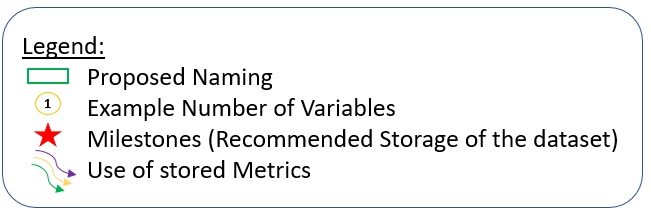
In the following I have created 4 diagrams that illustrate the development process of a machine learning algorithm. The complexity of the contents is constantly increasing.
Simple Development
Here we see a simple process for developing an algorithm for machine learning. Neither a filter method has given us a variable to exclude nor have we used a feature selection.
Development with Filter Methods
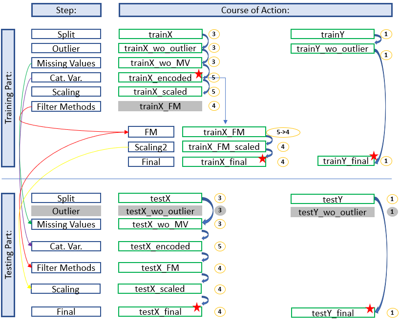
Here we see an overview where the filter methods have given us the option to exclude further variables.
For the trainings part this means that we have to access the stored dataset ‘trainX_encoded’ to apply the given filters and to do new feature scaling.
In the test part we are already richer in this information and can apply the filter methods before scaling.
Development with Feature Selection
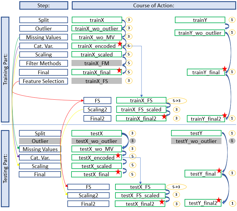
Here we see an architecture where we did feature selection after a training. This time a saved data set has to be reloaded and edited for the test part.
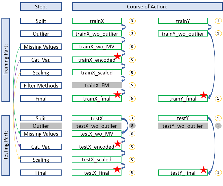
Development with Filter Methods and Feature Selection
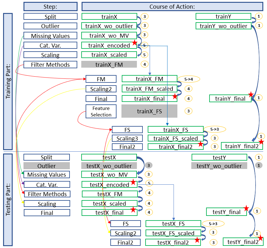
Here we see a final architecture where we have applied filter methods and excluded variables. Furthermore we have done feature selection after the first training.
The diagram shows which stored data sets have to be used to continue working and which naming conventions have to be applied to get a consistent and clear structure. In this way you always have a good overview and don’t get confused with the different objects / datasets etc. but always know where you are and in what state the dataset is.
The colored arrows show which metrics from which step were used in the test part and which data sets do not need to be renamed for which step (gray fields) because renaming would be pointless at this point. We can also see in the overview at which position (red stars) it is recommended to save the data set separately. This does not make sense for the first diagram (simple development), but if feature selection is still running you will be thankful that you made a backup copy at this point.
I hope the overviews help to make the development process easier or at least clearer for other data scientists in the future.
As already mentioned in some places in this publication, these guidelines can also be downloaded here: “DS Best Practice Guidlines for ML Model Development”.
8 Limitations
As in every publication there are a few limitations to mention.
- No statistical linear model was created to find out which predictors are significant.
- No further machine learning algorithms were trained for regression problems including hypter parameter tuning and tested to see if they might offer better performance.
- Not for all predictors average values (for later use) were saved.