1 Introduction
In my post Introduction to regression analysis and predictions I showed how to build regression models and also used evaluation metrics under chapter 4.
In this publication I would like to present metrics for regression analyses in more detail and show how they can be calculated.
For this post the dataset House Sales in King County, USA from the statistic platform “Kaggle” was used. You can download it from my “GitHub Repository”.
2 Loading the libraries and the data
import pandas as pd
import numpy as np

from sklearn.model_selection import train_test_split
from sklearn.preprocessing import StandardScaler

from sklearn.linear_model import LinearRegression

from sklearn import metrics
df = pd.read_csv('house_prices.csv')
df = df.drop(['id', 'date', 'yr_built', 'yr_renovated', 'zipcode', 'lat', 'long'], axis=1)
df.head()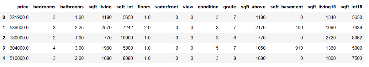
We will do the model training quick and dirty…
3 Data pre-processing
3.1 Train-Test Split
x = df.drop('price', axis=1)
y = df['price']

trainX, testX, trainY, testY = train_test_split(x, y, test_size = 0.2)
3.2 Scaling
sc=StandardScaler()

scaler = sc.fit(trainX)

trainX_scaled = scaler.transform(trainX)
testX_scaled = scaler.transform(testX)
4 Model fitting
lm = LinearRegression()
lm.fit(trainX_scaled, trainY)
5 Model Evaluation
y_pred = lm.predict(testX_scaled)Here are the prediction results:
df_results = pd.DataFrame({'Actual': testY, 'Predicted': y_pred})
df_results.head()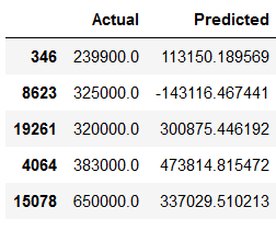
5.1 R²
The value R² tells us how much variance in the outcome variable can be explained by the predictors. Here: 60.6 %.
print('R²: ' + str(lm.score(trainX_scaled, trainY)))
5.2 Mean Absolute Error (MAE)
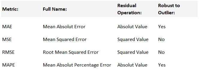
MAE stands for Mean Absolute Error and is probably the easiest regression error metric to understand. Here, each residual is calculated for each data point, taking only the absolute value of each point. This prevents positive and negative residuals from not canceling each other out. Then the average of all residuals is taken.
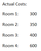
Here is a simple example:
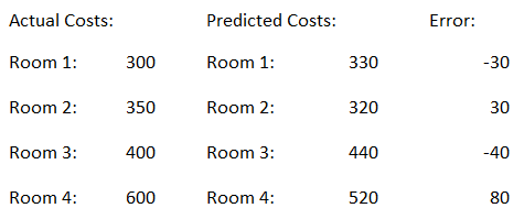
We have the actual cost of different rooms.
Now we contrast this with the Predicted Values.
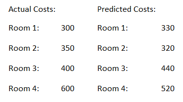
Now we calculate the error value as follows:
Error = Actual Costs - Predicted Costs
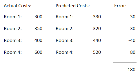
The absolute values are now summed up.
Now we calculate the mean value of the absolute error values.
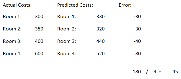
This is our measure of model quality. In this example, we can say that our model predictions are off by about €45.
Simply the MAE can be calculated with the following function:
print('Mean Absolute Error:', metrics.mean_absolute_error(testY, y_pred))
Of course, you could also calculate this value manually as in our example above.
df_results['error'] = df_results['Actual'] - df_results['Predicted']
df_results.head()
df_results['error_abs'] = df_results['error'].abs()
df_results.head()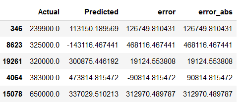
sum_error_abs = df_results['error_abs'].sum()
sum_error_abs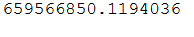
no_observations = len(df_results)
no_observations
mae = sum_error_abs / no_observations
mae
As we can see, this is the same value as above.
5.3 Mean Squared Error (MSE)
MSE stands for Mean Squared Error and is just like the Mean Absolute Error, but differs from it in that it squares the difference before summing instead of just taking the absolute value.
Since the difference is squared, the MSE will almost always be greater than the MAE. For this reason, the MSE cannot be directly compared to the MAE. Only the error metric of our model can be compared to that of a competing model. The effect of the quadratic term in the MSE equation is most apparent when there are outliers in the data set. Whereas in MAE this residual contributes proportionally to the total error, in MSE the error grows quadratically. Thus, existing outliers contribute to a much higher total error in MSE than they would in MAE.
print('Mean Squared Error:', metrics.mean_squared_error(testY, y_pred))
5.4 Root Mean Squared Error (RMSE)
RMSE stands for Root Mean Squared Error and this is the square root of the MSE. We know that the MSE is squared. Thus, its units do not match those of the original output. To convert the error metric back to similar units, the RMSE is used. This simplifies the interpretation again. Both MSE and RMSE are affected by outliers. Their common goal is to measure how large the residuals are distributed. Their values lie in the range between zero and positive infinity.
print('Root Mean Squared Error:', metrics.mean_squared_error(testY, y_pred, squared=False))
5.5 Mean Absolute Percentage Error (MAPE)
Another possible evaluation metric is the use of percentages. Here, each prediction is scaled against the value it is supposed to estimate. MAPE stands for Mean Absolute Percentage Error and is the percentage equivalent of MAE.
MAPE indicates how far the predictions of the model used deviate on average from the corresponding outputs. Both MAPE and MAE are accompanied by a clear interpretation, as percentages are easier to conceptualize for most people.
Both MAPE and MAE are robust to the effects of outliers. This is due to the use of absolute values.
print('Mean Absolute Percentage Error:', metrics.mean_absolute_percentage_error(testY, y_pred))
5.6 Summary of the Metrics
Here is again a summary of the metrics presented:
print('Mean Absolute Error:', metrics.mean_absolute_error(testY, y_pred))
print('Mean Squared Error:', metrics.mean_squared_error(testY, y_pred))
print('Root Mean Squared Error:', metrics.mean_squared_error(testY, y_pred, squared=False))
print('Mean Absolute Percentage Error:', metrics.mean_absolute_percentage_error(testY, y_pred))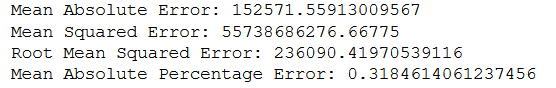
6 Conclusion
In this post, I showed which evaluation metrics you can use in a regression analysis and how to interpret and calculate them.