- 1 Introduction
- 2 Import the libraries
- 3 Data pre-processing
- 4 Descriptive Statistics
- 5 Simple CNN
- 6 CNN with Data Augmentation
- 7 Test Out of the Box Pictures
- 8 Conclusion
- 9 Link to the GitHub Repository
1 Introduction
So we got into Computer Vision and I described how to deal with image data in my last post Automate the Boring Stuff. Here I have also shown how to automatically split a dataset of images into a training, validation and test part.
I’ll barely cover that part in the post below and focus entirely on the topic at hand: How to classify the content of images using Convolutional Neural Networks.
What is a [Convolutional Neural(https://www.analyticsvidhya.com/blog/2016/04/deep-learning-computer-vision-introduction-convolution-neural-networks/) Network] (CNN)?
A CNN is is a deep learning neural network designed for processing structured arrays of data such as images. Convolutional Neural Networks are widely used in computer vision and have become the state of the art for many visual applications such as image classification. However, they can also be used for Recommender Systems, Natural Language Processing or Time Series Forecasting.
CNNs are very good at picking up on patterns in the input image, such as lines, gradients, circles or even eyes and faces. It is this property that makes CNNs so powerful for Computer Vision. A CNN is a feed-forward neural network. The power of a CNN comes from a special kind of layer called the convolutional layer. CNNs contain many convolutional layers stacked on top of each other, each one capable of recognizing more sophisticated shapes.

Source: DataFlair
In this publication I will show how to classify image data using a CNN. For this I used the images from the cats and dogs dataset from the statistics platform “Kaggle”. You can download the used data from my “GitHub Repository”.
2 Import the libraries
from preprocessing_CNN import Train_Validation_Test_Split

import numpy as np
import pandas as pd

import os
import shutil

import pickle as pk

import cv2
import matplotlib.pyplot as plt
%matplotlib inline

from keras import layers
from keras import models
from keras.callbacks import EarlyStopping, ModelCheckpoint

from keras.preprocessing.image import ImageDataGenerator
from keras.models import load_model
3 Data pre-processing
To get started with the training of a CNN, we first have to divide the data set into a training, validation and test part and determine some directories and metrics, so that we have less work later and can run through all processes fully automatically.
Please download the two folders cats and dogs from my “GitHub Repository” and navigate to the project’s root directory in the terminal. The notebook must be started from the location where the two files are stored.
3.1 Train-Validation-Test Split
In my post Automate the Boring Stuff I showed how to do such a split with image data automatically. I used exactly this syntax and packed it into a .py file to keep this notebook clear. You can also download this .py file from my “GitHub Repository”.
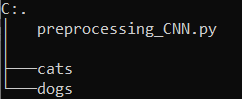
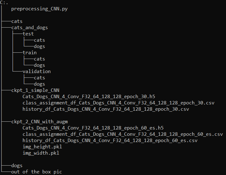
Place this file (preprocessing_CNN.py) next to the folders cats and dogs and start your Jupyter notebook from here.
Your folder structure should then look like this:
The function stored in the preprocessing_CNN.py file (Train_Validation_Test_Split) can be used as follows:
c_train, d_train, c_val, d_val, c_test, d_test = Train_Validation_Test_Split('cats', 'dogs')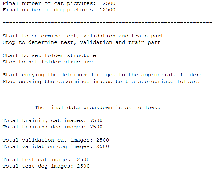
You only need to specify the two names of the folders in which the original image data is located or the entire path to the respective folders if you have stored the files somewhere else.
I have chosen the percentage distribution as follows:
- Trainings Part: 60%
- Validation Part: 20%
- Testing Part: 20%
Using the executed function, folders and subfolders are automatically created for the areas of training, validation and testing, and the image data is randomly divided according to the specified proportions.
As you can read in the function itself it returns 6 values:
- list_cats_training (int): List of randomly selected images for the training part of the first category
- list_dogs_training (int): List of randomly selected images for the training part of the second category
- list_cats_validation (int): List of randomly selected images for the validation part of the first category
- list_dogs_validation (int): List of randomly selected images for the validation part of the second category
- list_cats_test (int): List of randomly selected images for the test part of the first category
- list_dogs_test (int): List of randomly selected images for the test part of the second category
You don’t have to have these metrics output, but I use them later to determine some parameter settings of the neural network. You save as much as you can with smart programming.
3.2 Obtaining the lists of randomly selected images
To make the naming of the output of the function more meaningful I rename it accordingly
list_cats_training = c_train
list_dogs_training = d_train

list_cats_validation = c_val
list_dogs_validation = d_val

list_cats_test = c_test
list_dogs_test = d_test
3.3 Determination of the directories
Here I specify the path where the neural network can later find the data.
root_directory = os.getcwd()

train_dir = os.path.join(root_directory, 'cats_and_dogs\\train')
validation_dir = os.path.join(root_directory, 'cats_and_dogs\\validation')
test_dir = os.path.join(root_directory, 'cats_and_dogs\\test')
3.4 Obtain the total number of training, validation and test images
Here I’m not interested in reissuing the folder sizes but much more in getting the total number of images for the respective areas.
num_cats_img_train = len(list_cats_training)
num_dogs_img_train = len(list_dogs_training)

num_train_images_total = num_cats_img_train + num_dogs_img_train

print('Total training cat images: ' + str(num_cats_img_train))
print('Total training dog images: ' + str(num_dogs_img_train))
print()
print('Total training images: ' + str(num_train_images_total))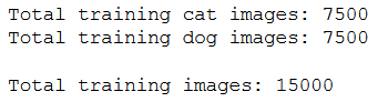
num_cats_img_validation = len(list_cats_validation)
num_dogs_img_validation = len(list_dogs_validation)

num_validation_images_total = num_cats_img_validation + num_dogs_img_validation

print('Total validation cat images: ' + str(num_cats_img_validation))
print('Total validation dog images: ' + str(num_dogs_img_validation))
print()
print('Total validation images: ' + str(num_validation_images_total))
num_cats_img_test = len(list_cats_test)
num_dogs_img_test = len(list_dogs_test)

num_test_images_total = num_cats_img_test + num_dogs_img_test

print('Total test cat images: ' + str(num_cats_img_test))
print('Total test dog images: ' + str(num_dogs_img_test))
print()
print('Total test images: ' + str(num_test_images_total))
The folder structure should now look like this:

4 Descriptive Statistics
Here are a few more descriptive statistics on the images we have available to us:
root_directory = os.getcwd()
train_files_cats_dir = os.path.join(root_directory, 'cats_and_dogs\\train\\cats')

height, width = [], []

fnames = ['cat{}.jpg'.format(i) for i in list_cats_training]
for fname in fnames:
    img_name = os.path.join(train_files_cats_dir, fname)
    img = cv2.imread(img_name)
    height.append(img.shape[0])
    width.append(img.shape[1])

plt.scatter(height,width, s=1)
plt.xlabel('Height', fontsize=16)
plt.ylabel('Width', fontsize=16)
plt.title('Scatter Plot of Height and Width of cat train images')
plt.show() 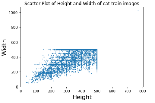
plt.hist(height,bins = 50, alpha=0.5)
plt.hist(width,bins = 50,alpha=0.5)
plt.axis([0,600,0,4000])
plt.xlabel('Height/Width', fontsize=16)
plt.ylabel('Num of Images', fontsize=16)
plt.title('Variation of image sizes within dataset')
plt.show()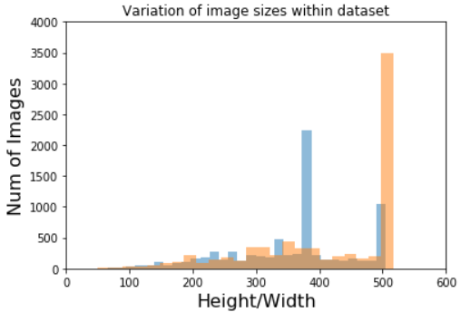
root_directory = os.getcwd()
train_files_dogs_dir = os.path.join(root_directory, 'cats_and_dogs\\train\\dogs')

height, width = [], []

fnames = ['dog{}.jpg'.format(i) for i in list_dogs_training]
for fname in fnames:
    img_name = os.path.join(train_files_dogs_dir, fname)
    img = cv2.imread(img_name)
    height.append(img.shape[0])
    width.append(img.shape[1])

plt.scatter(height,width, s=1)
plt.xlabel('Height', fontsize=16)
plt.ylabel('Width', fontsize=16)
plt.title('Scatter Plot of Height and Width of dog train images')
plt.show() 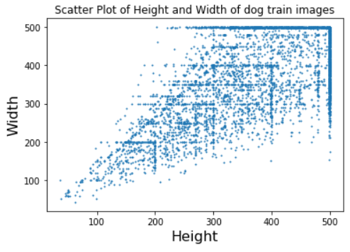
plt.hist(height,bins = 50, alpha=0.5)
plt.hist(width,bins = 50,alpha=0.5)
plt.axis([0,600,0,4000])
plt.xlabel('Height/Width', fontsize=16)
plt.ylabel('Num of Images', fontsize=16)
plt.title('Variation of image sizes within dataset')
plt.show()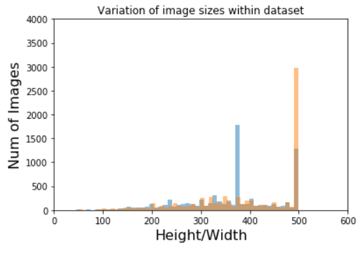
5 Simple CNN
5.1 Name Definitions
I always want to save the created models right away. For this purpose, I specify the name of the folder in which the future model is to be saved and the name that the model itself is to receive.
checkpoint_no = 'ckpt_1_simple_CNN'
model_name = 'Cats_Dogs_CNN_4_Conv_F32_64_128_128_epoch_30'
5.2 Parameter Settings
First, I determine the height and width of the images as they are to be read into the model. This then results in the input_shape. The 3 stands for the image depth. Since we are dealing with colored images, we have a depth of 3 for red, green and blue (RGB).
batch_size
Batch Size determines the number of samples in each mini-batch. Its maximum is the number of all samples, which makes the gradient descent accurate, the loss will decrease towards the minimum if the learning rate is small enough, but the iterations are slower. Its minimum is 1, resulting in a stochastic gradient descent: Fast, but the direction of the gradient step is based on one example only, the loss can jump around. Batch Size allows setting between the two extremes: exact gradient direction and fast iteration. Also, the maximum value for Batch Size may be limited if your model and dataset do not fit in the available (GPU) memory.
steps_per_epoch
Steps per Epoch is the number of batch iterations before a training epoch is considered complete. If you have a fixed-size training dataset, you can ignore it, but it can be useful if you have a huge dataset or if you generate random data extensions on the fly, i.e. if your training dataset has a (generated) infinite size. If you have the time to go through your entire training dataset, I recommend skipping this parameter.
validation_steps and test_steps
These two parameter are similar to Steps per Epoch but on the validation and test data set instead on the training data. If you have the time to go through your whole validation and test data set I recommend to skip this parameter as well.
n_epochs
Number of epochs how often a complete run should be performed. One epoch is when an entire dataset is passed forward and backward through the neural network only once.
We can divide a dataset of 2000 examples into Batch Size of 500 then it will take 4 Steps per Epoch to complete 1 epoch.
Here we see the reason why I have some metrics returned from the Train_Validation_Test_Split function. After I have set a batch size of 32, the total amount of 15,000 training images results in 468 steps per epoch, so that all images were seen once per epoch.
The same is true for validation and test steps.
img_height = 150
img_width = 150
input_shape = (img_height, img_width, 3)

n_batch_size = 32

n_steps_per_epoch = int(num_train_images_total / n_batch_size)
n_validation_steps = int(num_validation_images_total / n_batch_size)
n_test_steps = int(num_test_images_total / n_batch_size)

n_epochs = 30

print('Input Shape: '+'('+str(img_height)+', '+str(img_width)+', ' + str(3)+')')
print('Batch Size: ' + str(n_batch_size))
print()
print('Steps per Epoch: ' + str(n_steps_per_epoch))
print()
print('Validation Steps: ' + str(n_validation_steps))
print('Test Steps: ' + str(n_test_steps))
print()
print('Number of Epochs: ' + str(n_epochs))
I will always need this information with the ImageDataGenerators as well. Therefore, it has become a best practice to define the parameters once based on the calculations of the metrics from the split function.
5.3 Instantiating a small CNN
5.3.1 Layer Structure
model = models.Sequential()
model.add(layers.Conv2D(32, (3, 3), activation='relu',input_shape=input_shape))
model.add(layers.MaxPooling2D((2, 2)))

model.add(layers.Conv2D(64, (3, 3), activation='relu'))
model.add(layers.MaxPooling2D((2, 2)))

model.add(layers.Conv2D(128, (3, 3), activation='relu'))
model.add(layers.MaxPooling2D((2, 2)))

model.add(layers.Conv2D(128, (3, 3), activation='relu'))
model.add(layers.MaxPooling2D((2, 2)))

model.add(layers.Flatten())

model.add(layers.Dense(512, activation='relu'))
model.add(layers.Dense(1, activation='sigmoid'))
I set the last Dense Layer to 1 and chose ‘sigmoid’ as the activation function, since this is a binary classification problem.
model.summary()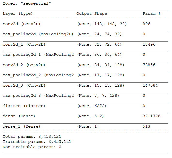
If you want to know how the total number of parameters is calculated, see this post.
5.3.2 Configuring the model for training
model.compile(loss='binary_crossentropy',
              optimizer='adam',
              metrics=['accuracy'])
5.3.3 Using ImageDataGenerator
train_datagen = ImageDataGenerator(rescale=1./255)
validation_datagen = ImageDataGenerator(rescale=1./255)


train_generator = train_datagen.flow_from_directory(
        train_dir,
        target_size=(img_height, img_width),
        batch_size=n_batch_size,
        class_mode='binary')

validation_generator = validation_datagen.flow_from_directory(
        validation_dir,
        target_size=(img_height, img_width),
        batch_size=n_batch_size,
        class_mode='binary')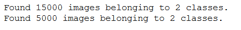
5.4 Callbacks
The Keras library offers the option of callbacks. Personally, I pretty much always use two of them:
ModelCheckpoint gives me the possibility to automatically save models measured by a defined metric (here validation loss) if this metric has improved after an epoch.
EarlyStopping protects me from unnecessary further training of the model if a particular metric does not continue to improve over a number of n epochs. In such a case, the model training would be automatically aborted.
But there are other useful callbacks like ReduceLROnPlateau. Here, the learning rate would automatically reduce if a metric stopped improving.
In the following I first used only ModelCheckpoint but in the model training with Data Augmentation under chapter 6.4 I also included EarlyStopping.
# Prepare a directory to store all the checkpoints.
checkpoint_dir = './'+ checkpoint_no
if not os.path.exists(checkpoint_dir):
    os.makedirs(checkpoint_dir)
keras_callbacks = [ModelCheckpoint(filepath = checkpoint_dir + '/' + model_name,
monitor='val_loss', save_best_only=True, mode='auto')]5.5 Fitting the model
After we have already determined the parameters, we now benefit from the fact that we no longer have to make any manual entries.
history = model.fit(
      train_generator,
      steps_per_epoch=n_steps_per_epoch,
      epochs=n_epochs,
      validation_data=validation_generator,
      validation_steps=n_validation_steps,
      callbacks=keras_callbacks)
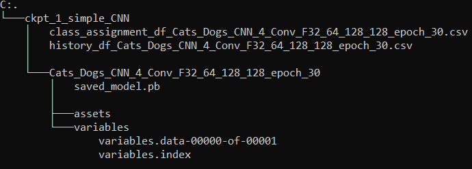
After model training, your folder structure should look like this:

Here we see that our callback (ModelCheckpoint) has automatically created a folder ‘ckpt_1_simple_CNN’ (the name I gave in chapter 5.1) with a subfolder containing the automatically saved model.
5.6 Obtaining the best model values
By using the callback ModelCheckpoint the model was saved which had the lowest validaton loss. But what exactly were the values of this model? With the following code I have the possibility to display the values per epoch. And with this dataframe I also have the possibility to display the values for the model that was automatically saved.
hist_df = pd.DataFrame(history.history)
hist_df['epoch'] = hist_df.index + 1
cols = list(hist_df.columns)
cols = [cols[-1]] + cols[:-1]
hist_df = hist_df[cols]
hist_df.to_csv(checkpoint_no + '/' + 'history_df_' + model_name + '.csv')
hist_df.head()
values_of_best_model = hist_df[hist_df.val_loss == hist_df.val_loss.min()]
values_of_best_model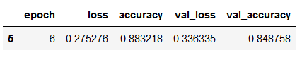
Since I will possibly train several models in several notebooks at the same time, it is advisable at this point to save the dataframe shown above as a .csv file in order to be able to refer to it again at a later time, for example to compare the model performance of the best models.
I have now saved the history values in my ModelCheckpoint folder. This folder now looks like this:

5.7 Obtaining class assignments
In addition to the metric values achieved per epoch during model training, it is also advisable to have the assigned class distribution output and to save this information as a .csv file so that you can refer to it again later.
class_assignment = train_generator.class_indices

df = pd.DataFrame([class_assignment], columns=class_assignment.keys())
df_stacked = df.stack()
df_temp = pd.DataFrame(df_stacked).reset_index().drop(['level_0'], axis=1)
df_temp.columns = ['Category', 'Allocated Number']
df_temp.to_csv(checkpoint_no + '/' + 'class_assignment_df_' + model_name + '.csv')

print('Class assignment:', str(class_assignment))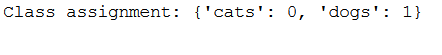
Both files (the history values and the class assignments) are now stored in my ModelCheckpoint folder. This folder now looks like this:
5.8 Validation
In the following I will generate two graphs showing the training and validation accuracy on the one hand and the training and validation loss on the other hand.
acc = history.history['accuracy']
val_acc = history.history['val_accuracy']
loss = history.history['loss']
val_loss = history.history['val_loss']

epochs = range(1, len(acc) + 1)

plt.plot(epochs, acc, 'bo', label='Training acc')
plt.plot(epochs, val_acc, 'b', label='Validation acc')
plt.title('Training and validation accuracy')
plt.legend()

plt.figure()

plt.plot(epochs, loss, 'bo', label='Training loss')
plt.plot(epochs, val_loss, 'b', label='Validation loss')
plt.title('Training and validation loss')
plt.legend()

plt.show()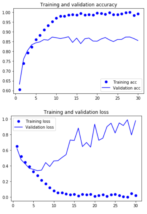
The graphs clearly show that we have a problem with overfitting.
5.9 Load best model
As you can see from the current folder structure shown above (Chapter 5.7), the automatically created subfolders inside the ModelCheckpoint folder are not that great. The best model was saved as a .pb file and did not get a proper naming.
I want my final model to be saved with appropriate naming under the created ModelCheckpoint folder. Since I am aiming for this tidy approach I will load the .pb model below, save it as an .h5 file and delete the unnecessary folders.
# Loading the automatically saved model
model_reloaded = load_model(checkpoint_no + '/' + model_name)

# Saving the best model in the correct path and format
root_directory = os.getcwd()
checkpoint_dir = os.path.join(root_directory, checkpoint_no)
model_name_temp = os.path.join(checkpoint_dir, model_name + '.h5')
model_reloaded.save(model_name_temp)

# Deletion of the automatically created folder under Model Checkpoint File.
folder_name_temp = os.path.join(checkpoint_dir, model_name)
shutil.rmtree(folder_name_temp, ignore_errors=True)
Our ModelCheckpoint folder should then look like this:

The overall folder structure should look like this:

As a final step we load the saved .h5 model.
best_model = load_model(model_name_temp)5.10 Model Testing
With the .h5 model reloaded, let’s now check the performance of the CNN using the test data.
test_datagen = ImageDataGenerator(rescale=1./255)

test_generator = test_datagen.flow_from_directory(
        test_dir,
        target_size=(img_height, img_width),
        batch_size=n_batch_size,
        class_mode='binary')

test_loss, test_acc = best_model.evaluate(test_generator, steps=n_test_steps)
print()
print('Test Accuracy:', test_acc)
As expected, the performance is not that good yet. Therefore, we perform another model training.
6 CNN with Data Augmentation
Data Augmentation is a nice way to prevent overfitting, especially in computer vision. Here the amount of training is increased by rotating, stretching and other modification processes of the images.
Most steps and settings remain the same. Therefore, I will only discuss noteworthy changes in the following.
6.1 Name Definitions
checkpoint_no = 'ckpt_2_CNN_with_augm'
model_name = 'Cats_Dogs_CNN_4_Conv_F32_64_128_128_epoch_60_es'
6.2 Parameter Settings
img_height = 150
img_width = 150
input_shape = (img_height, img_width, 3)

n_batch_size = 64

n_steps_per_epoch = int(num_train_images_total / n_batch_size)
n_validation_steps = int(num_validation_images_total / n_batch_size)
n_test_steps = int(num_test_images_total / n_batch_size)

n_epochs = 60

print('Input Shape: '+'('+str(img_height)+', '+str(img_width)+', ' + str(3)+')')
print('Batch Size: ' + str(n_batch_size))
print()
print('Steps per Epoch: ' + str(n_steps_per_epoch))
print()
print('Validation Steps: ' + str(n_validation_steps))
print('Test Steps: ' + str(n_test_steps))
print()
print('Number of Epochs: ' + str(n_epochs))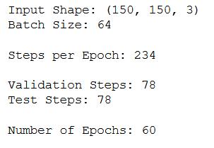
6.3 Instantiating a CNN with Data Augmentation
6.3.1 Layer Structure
I have added an additional dropout layer here, which should also counteract overfittig.
model = models.Sequential()
model.add(layers.Conv2D(32, (3, 3), activation='relu',input_shape=input_shape))
model.add(layers.MaxPooling2D((2, 2)))

model.add(layers.Conv2D(64, (3, 3), activation='relu'))
model.add(layers.MaxPooling2D((2, 2)))

model.add(layers.Conv2D(128, (3, 3), activation='relu'))
model.add(layers.MaxPooling2D((2, 2)))

model.add(layers.Conv2D(128, (3, 3), activation='relu'))
model.add(layers.MaxPooling2D((2, 2)))

model.add(layers.Flatten())

model.add(layers.Dropout(0.5))

model.add(layers.Dense(512, activation='relu'))
model.add(layers.Dense(1, activation='sigmoid'))
model.summary()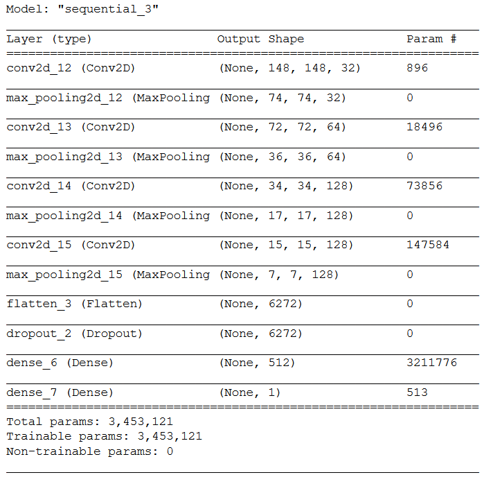
6.3.2 Configuring the model for training
model.compile(loss='binary_crossentropy',
              optimizer='adam',
              metrics=['accuracy'])
6.3.3 Using ImageDataGenerator with data augmentation
train_datagen = ImageDataGenerator(
    rescale=1./255,
    rotation_range=40,
    width_shift_range=0.2,
    height_shift_range=0.2,
    shear_range=0.2,
    zoom_range=0.2,
    horizontal_flip=True,)

validation_datagen = ImageDataGenerator(rescale=1./255)


train_generator = train_datagen.flow_from_directory(
        train_dir,
        target_size=(img_height, img_width),
        batch_size=n_batch_size,
        class_mode='binary')

validation_generator = validation_datagen.flow_from_directory(
        validation_dir,
        target_size=(img_height, img_width),
        batch_size=n_batch_size,
        class_mode='binary')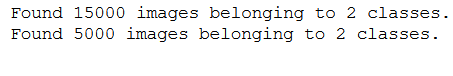
6.4 Callbacks
As previously announced, I use not only the ModelCheckpoint callback here but also the EarlyStopping. With EarlyStopping I also monitor the validation loss and say with patience=5, if this value does not improve over a number of 5 epochs, please stop the model training.
# Prepare a directory to store all the checkpoints.
checkpoint_dir = './'+ checkpoint_no
if not os.path.exists(checkpoint_dir):
    os.makedirs(checkpoint_dir)
keras_callbacks = [ModelCheckpoint(filepath = checkpoint_dir + '/' + model_name,
monitor='val_loss', save_best_only=True, mode='auto'),
EarlyStopping(monitor='val_loss', patience=5, mode='auto',
min_delta = 0, verbose=1)]6.5 Fitting the model
history = model.fit(
      train_generator,
      steps_per_epoch=n_steps_per_epoch,
      epochs=n_epochs,
      validation_data=validation_generator,
      validation_steps=n_validation_steps,
      callbacks=keras_callbacks)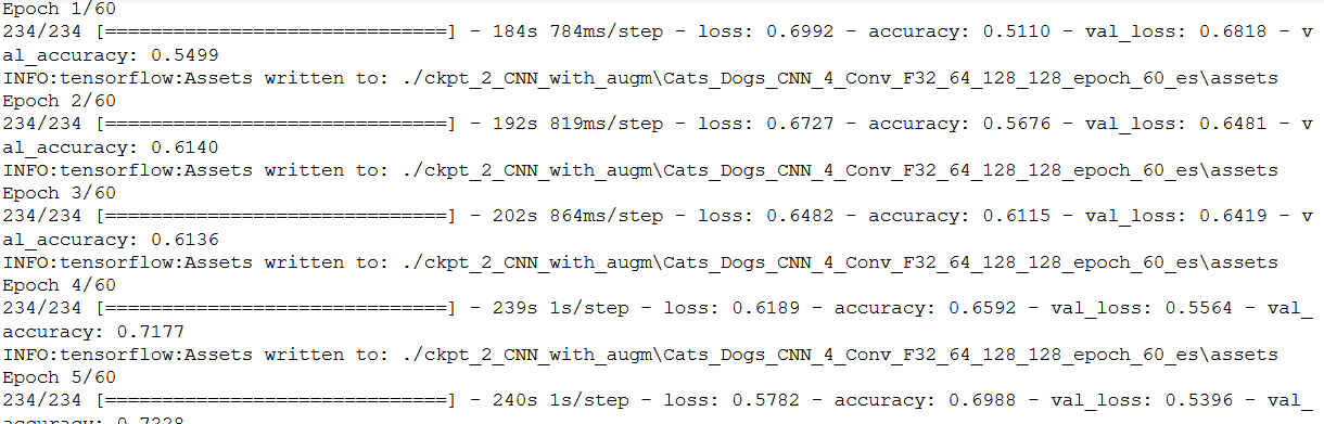
6.6 Obtaining the best model values
hist_df = pd.DataFrame(history.history)
hist_df['epoch'] = hist_df.index + 1
cols = list(hist_df.columns)
cols = [cols[-1]] + cols[:-1]
hist_df = hist_df[cols]
hist_df.to_csv(checkpoint_no + '/' + 'history_df_' + model_name + '.csv')
hist_df.head()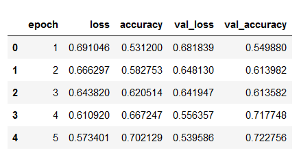
values_of_best_model = hist_df[hist_df.val_loss == hist_df.val_loss.min()]
values_of_best_model
6.7 Obtaining class assignments
class_assignment = train_generator.class_indices

df = pd.DataFrame([class_assignment], columns=class_assignment.keys())
df_stacked = df.stack()
df_temp = pd.DataFrame(df_stacked).reset_index().drop(['level_0'], axis=1)
df_temp.columns = ['Category', 'Allocated Number']
df_temp.to_csv(checkpoint_no + '/' + 'class_assignment_df_' + model_name + '.csv')

print('Class assignment:', str(class_assignment))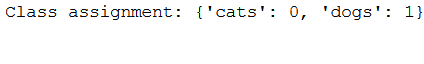
6.8 Validation
acc = history.history['accuracy']
val_acc = history.history['val_accuracy']
loss = history.history['loss']
val_loss = history.history['val_loss']

epochs = range(1, len(acc) + 1)

plt.plot(epochs, acc, 'bo', label='Training acc')
plt.plot(epochs, val_acc, 'b', label='Validation acc')
plt.title('Training and validation accuracy')
plt.legend()

plt.figure()

plt.plot(epochs, loss, 'bo', label='Training loss')
plt.plot(epochs, val_loss, 'b', label='Validation loss')
plt.title('Training and validation loss')
plt.legend()

plt.show()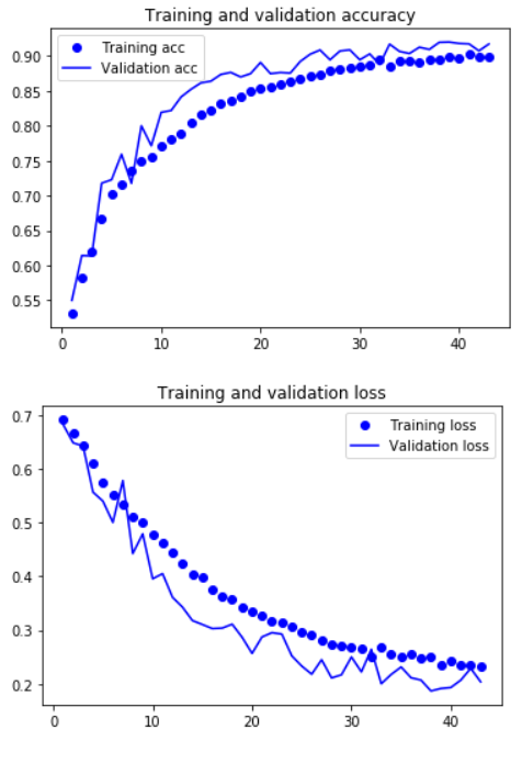
That looks a lot better.
6.9 Load best model
# Loading the automatically saved model
model_reloaded = load_model(checkpoint_no + '/' + model_name)

# Saving the best model in the correct path and format
root_directory = os.getcwd()
checkpoint_dir = os.path.join(root_directory, checkpoint_no)
model_name_temp = os.path.join(checkpoint_dir, model_name + '.h5')
model_reloaded.save(model_name_temp)

# Deletion of the automatically created folder under Model Checkpoint File.
folder_name_temp = os.path.join(checkpoint_dir, model_name)
shutil.rmtree(folder_name_temp, ignore_errors=True)
best_model = load_model(model_name_temp)6.10 Model Testing
test_datagen = ImageDataGenerator(rescale=1./255)

test_generator = test_datagen.flow_from_directory(
        test_dir,
        target_size=(img_height, img_width),
        batch_size=n_batch_size,
        class_mode='binary')

test_loss, test_acc = best_model.evaluate(test_generator, steps=n_test_steps)
print()
print('Test Accuracy:', test_acc)
As we can see, the use of Data Augmentation and an increased number of training epochs has brought the Accuracy to over 91%.
Since this will be our final model, it is advisable to save the following two metrics that we used for this model training:
- img_height
- img_width
Why do we store these two values separately?
We want to use our model later to predict completely new images. To be able to do this, we need to put the images we read in later into the same format as the model training took place. In this case we have resized all images to 150x150. This is exactly what we will do with future images to be able to predict them.
pk.dump(img_height, open(checkpoint_dir+ '\\' +'img_height.pkl', 'wb'))
pk.dump(img_width, open(checkpoint_dir+ '\\' +'img_width.pkl', 'wb'))
I’m sure we can increase the accuracy again by either increasing the patience value in EarlyStopping or omitting EarlyStopping altogether, so in both cases the model training runs for an even longer time.
In our case, the best model from epoch 38 was saved.
Feel free to try this out for yourself and report back to me with your results.
The final folder structure should now look like this:
7 Test Out of the Box Pictures
Last but not least, I always test the final model again with completely different images that were not included in the main data sets. To do this, we load the categories and some of the training metrics used.
# Load the categories
df = pd.read_csv('ckpt_2_CNN_with_augm/class_assignment_df_Cats_Dogs_CNN_4_Conv_F32_64_128_128_epoch_60_es.csv')
df = df.sort_values(by='Allocated Number', ascending=True)
CATEGORIES = df['Category'].to_list()

# Load the used image height and width
img_height_reload = pk.load(open("ckpt_2_CNN_with_augm/img_height.pkl",'rb'))
img_width_reload = pk.load(open("ckpt_2_CNN_with_augm/img_width.pkl",'rb'))


print('CATEGORIES : ' + str(CATEGORIES))
print()
print('Used image height: ' + str(img_height_reload))
print('Used image width: ' + str(img_width_reload))
Look at the results:
img_pred = cv2.imread('out of the box pic/test_cat_pic_1.jpg')

print(plt.imshow(cv2.cvtColor(img_pred, cv2.COLOR_BGR2RGB)))

img_pred = cv2.resize(img_pred,(img_height_reload,img_width_reload))
img_pred = np.reshape(img_pred,[1,img_height_reload,img_width_reload,3])

classes = (best_model.predict(img_pred) > 0.5).astype("int32")

print()
print('------------------------------------')
print('Predicted Class: ' + CATEGORIES[int(classes[0])])
print('------------------------------------')
img_pred = cv2.imread('out of the box pic/test_cat_pic_2.jpg')

print(plt.imshow(cv2.cvtColor(img_pred, cv2.COLOR_BGR2RGB)))

img_pred = cv2.resize(img_pred,(img_height_reload,img_width_reload))
img_pred = np.reshape(img_pred,[1,img_height_reload,img_width_reload,3])

classes = (best_model.predict(img_pred) > 0.5).astype("int32")

print()
print('------------------------------------')
print('Predicted Class: ' + CATEGORIES[int(classes[0])])
print('------------------------------------')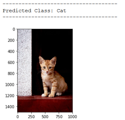
img_pred = cv2.imread('out of the box pic/test_dog_pic_1.jpg')

print(plt.imshow(cv2.cvtColor(img_pred, cv2.COLOR_BGR2RGB)))

img_pred = cv2.resize(img_pred,(img_height_reload,img_width_reload))
img_pred = np.reshape(img_pred,[1,img_height_reload,img_width_reload,3])

classes = (best_model.predict(img_pred) > 0.5).astype("int32")

print()
print('------------------------------------')
print('Predicted Class: ' + CATEGORIES[int(classes[0])])
print('------------------------------------')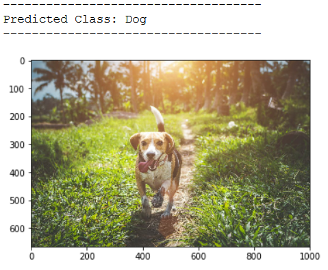
img_pred = cv2.imread('out of the box pic/test_dog_pic_2.jpg')

print(plt.imshow(cv2.cvtColor(img_pred, cv2.COLOR_BGR2RGB)))

img_pred = cv2.resize(img_pred,(img_height_reload,img_width_reload))
img_pred = np.reshape(img_pred,[1,img_height_reload,img_width_reload,3])

classes = (best_model.predict(img_pred) > 0.5).astype("int32")

print()
print('------------------------------------')
print('Predicted Class: ' + CATEGORIES[int(classes[0])])
print('------------------------------------')
8 Conclusion
In this post I have talked in detail about the use of Convolutional Neural Networks and how they can be used to solve binary classification problems with images.
9 Link to the GitHub Repository
Here is the link to my GitHub repository where I have listed all necessary steps: Computer Vision: CNN for binary Classification
References
The content of the entire post was created using the following sources:
Chollet, F. (2018). Deep learning with Python (Vol. 361). New York: Manning.