1 Introduction
Neural networks can be used not only for “univariate time series”. We can also incorporate other predictors into the model with their help. This is what this post is about.
For this post the dataset Metro_Interstate_Traffic_Volume from the statistic platform “Kaggle” was used. You can download it from my “GitHub Repository”.
2 Import the libraries and the data
import pandas as pd
import numpy as np

from sklearn import preprocessing
from sklearn import metrics
import tensorflow as tf
from xgboost import XGBRegressor

import matplotlib.pyplot as plt

import warnings
warnings.filterwarnings("ignore")
df = pd.read_csv('Metro_Interstate_Traffic_Volume.csv')
print(df.shape)
df.head()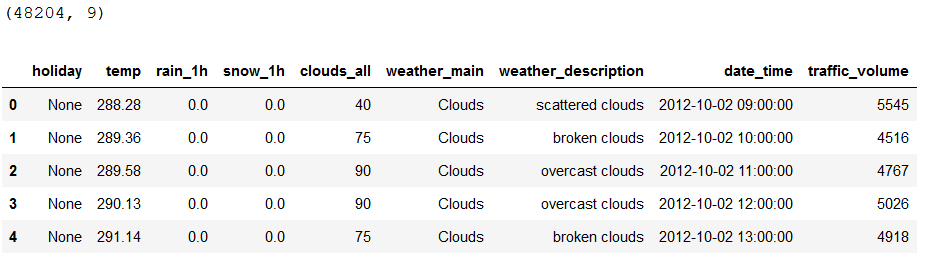
The variable ‘traffic_volume’ will be our target variable again.
3 Definition of required functions
def mean_absolute_percentage_error_func(y_true, y_pred):
    '''
    Calculate the mean absolute percentage error as a metric for evaluation

    Args:
        y_true (float64): Y values for the dependent variable (test part), numpy array of floats
        y_pred (float64): Predicted values for the dependen variable (test parrt), numpy array of floats

    Returns:
        Mean absolute percentage error
    '''
    y_true, y_pred = np.array(y_true), np.array(y_pred)
    return np.mean(np.abs((y_true - y_pred) / y_true)) * 100
def timeseries_evaluation_metrics_func(y_true, y_pred):
'''
Calculate the following evaluation metrics:
- MSE
- MAE
- RMSE
- MAPE
- R²
Args:
y_true (float64): Y values for the dependent variable (test part), numpy array of floats
y_pred (float64): Predicted values for the dependen variable (test parrt), numpy array of floats
Returns:
MSE, MAE, RMSE, MAPE and R²
'''
print('Evaluation metric results: ')
print(f'MSE is : {metrics.mean_squared_error(y_true, y_pred)}')
print(f'MAE is : {metrics.mean_absolute_error(y_true, y_pred)}')
print(f'RMSE is : {np.sqrt(metrics.mean_squared_error(y_true, y_pred))}')
print(f'MAPE is : {mean_absolute_percentage_error_func(y_true, y_pred)}')
print(f'R2 is : {metrics.r2_score(y_true, y_pred)}',end='\n\n')def multiple_data_prep_func(predictors, target, start, end, window, horizon):
'''
Prepare univariate data that is suitable for a time series
Args:
predictors (float64): Scaled values for the predictors, numpy array of floats
target (float64): Scaled values for the target variable, numpy array of floats
start (int): Start point of range, integer
end (int): End point of range, integer
window (int): Number of units to be viewed per step, integer
horizon (int): Number of units to be predicted, integer
Returns:
X (float64): Generated X-values for each step, numpy array of floats
y (float64): Generated y-values for each step, numpy array of floats
'''
X = []
y = []
start = start + window
if end is None:
end = len(predictors) - horizon
for i in range(start, end):
indices = range(i-window, i)
X.append(predictors[indices])
indicey = range(i+1, i+1+horizon)
y.append(target[indicey])
return np.array(X), np.array(y)4 Data pre-processing
4.1 Drop Duplicates
df = df.drop_duplicates(subset=['date_time'], keep=False)

df.shape
4.2 Feature Encoding
We have three categorical variables (‘holiday’, ‘weather_main’ and ‘weather_description’) which need to be coded. We use the get_dummies function for this which does the same as One Hot Encoding from Scikit Learn.
# Encode feature 'holiday'
dummy_holiday = pd.get_dummies(df['holiday'], prefix="holiday")
column_name = df.columns.values.tolist()
column_name.remove('holiday')
df = df[column_name].join(dummy_holiday)

# Encode feature 'weather_main'
dummy_weather_main = pd.get_dummies(df['weather_main'], prefix="weather_main")
column_name = df.columns.values.tolist()
column_name.remove('weather_main')
df = df[column_name].join(dummy_weather_main)


# Encode feature 'weather_description'
dummy_weather_description = pd.get_dummies(df['weather_description'], prefix="weather_description")
column_name = df.columns.values.tolist()
column_name.remove('weather_description')
df = df[column_name].join(dummy_weather_description)

# Print final dataframe
print()
print('Shape of new dataframe: ' + str(df.shape))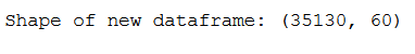
Now we have increased the number of features from our dataset from 9 to 60.
4.3 Check for Feature Importance
Since not all features are relevant, we can check the Feature Importance at this point. We use XGBoost for this, since this algorithm has a very strong performance for our problem.
column_names_predictors = df.columns.values.tolist()

# Exclude target variable and date_time
column_names_predictors.remove('traffic_volume')
column_names_predictors.remove('date_time')

column_name_criterium = 'traffic_volume'

print('Length of remaining predictors: ' + str(len(column_names_predictors)))
print()
print('Target Variable: ' + str(column_name_criterium))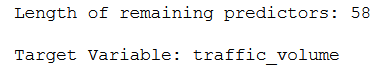
model = XGBRegressor()
model.fit(df[column_names_predictors],df[column_name_criterium])
Let’s output the features with the corresponding score value, which have been retained by XGBoost.
feature_important = model.get_booster().get_score(importance_type='gain')
keys = list(feature_important.keys())
values = list(feature_important.values())

data = pd.DataFrame(data=values, index=keys, columns=["score"]).sort_values(by = "score", ascending=False)
data.plot(kind='barh')

print()
print('Length of remaining predictors after XGB: ' + str(len(data)))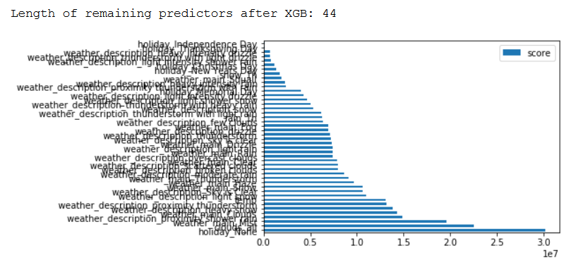
The calculation of the respective score can be set differently depending on the importance_type. Here is an overview of which calculation types are available:
weight- the number of times a feature is used to split the data across all trees.gain- the average gain across all splits the feature is used in.cover- the average coverage across all splits the feature is used in.total_gain- the total gain across all splits the feature is used in.total_cover- the total coverage across all splits the feature is used in.
Let’s create our final dataframe:
# Get column names of remaining predictors after XGB
features_to_keep = list(data.index)
# Append name of target variable
features_to_keep.append(column_name_criterium)

# Create final dataframe
final_df = df[features_to_keep]

print()
print('Length of features_to_keep: ' + str(len(features_to_keep)))
print('(includes 44 predictors and the target variable)')
print()
print('Shape of final dataframe: ' + str(final_df.shape))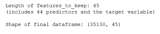
4.4 Generate Test Set
Of course, we again need a test set that was not seen in any way by the created neural networks.
test_data = final_df.tail(10)

final_df = final_df.drop(final_df.tail(10).index)

final_df.shape
4.5 Feature Scaling
scaler_x = preprocessing.MinMaxScaler()
scaler_y = preprocessing.MinMaxScaler()

# Here we scale the predictors
x_scaled = scaler_x.fit_transform(final_df.drop(column_name_criterium, axis=1))
# Here we scale the criterium
y_scaled = scaler_y.fit_transform(final_df[[column_name_criterium]])
4.6 Train-Validation Split
In the last post about time series analysis with neural networks I presented two methods:
- Single Step Style
- Horizon Style
The single step style is not possible for neural networks with multiple predictors. Why not ? See here:

Here in the Single Step Style at univariate Time Series, we can use the prediction made before for the one that follows.
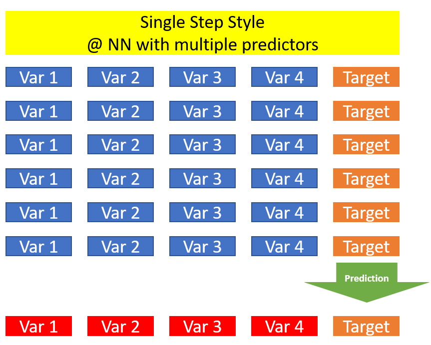
If we now have multiple predictors, we can determine the one value for the target variable, but we do not have predicted values for our predictors on the basis of which we can make the further predictions.
For this reason, we must limit ourselves to Horizon Style at this point.
# Here we allow the model to see / train the last 48 observations
multi_hist_window_hs = 48
# Here we try to predict the following 10 observations
# Must be the same length as the test_data !
horizon_hs = 10
train_split_hs = 30000

x_train_multi_hs, y_train_multi_hs = multiple_data_prep_func(x_scaled, y_scaled,
                                                             0, train_split_hs,
                                                             multi_hist_window_hs, horizon_hs)

x_val_multi_hs, y_val_multi_hs= multiple_data_prep_func(x_scaled, y_scaled,
                                                        train_split_hs, None,
                                                        multi_hist_window_hs, horizon_hs)
print ('Length of first Single Window:')
print (len(x_train_multi_hs[0]))
print()
print ('Target horizon:')
print (y_train_multi_hs[0])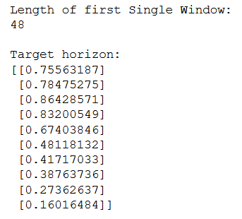
4.7 Prepare training and test data using tf
BATCH_SIZE_hs = 256
BUFFER_SIZE_hs = 150

train_multi_hs = tf.data.Dataset.from_tensor_slices((x_train_multi_hs, y_train_multi_hs))
train_multi_hs = train_multi_hs.cache().shuffle(BUFFER_SIZE_hs).batch(BATCH_SIZE_hs).repeat()

validation_multi_hs = tf.data.Dataset.from_tensor_slices((x_val_multi_hs, y_val_multi_hs))
validation_multi_hs = validation_multi_hs.batch(BATCH_SIZE_hs).repeat()
5 Neural Networks with mult. predictors
In the following, I will again use several types of neural networks, which are possible for time series analysis, to check which type of neural network fits our data best.
The following networks will be used:
- LSTM
- Bidirectional LSTM
- GRU
- Encoder Decoder LSTM
- CNN
To save me more lines of code later, I’ll set a few parameters for the model training at this point:
n_steps_per_epoch = 117
n_validation_steps = 20
n_epochs = 100
5.1 LSTM
Define Layer Structure
model = tf.keras.models.Sequential([
    tf.keras.layers.LSTM(100, input_shape=x_train_multi_hs.shape[-2:],return_sequences=True),
    tf.keras.layers.Dropout(0.2),
    tf.keras.layers.LSTM(units=100,return_sequences=False),
    tf.keras.layers.Dropout(0.2),
    tf.keras.layers.Dense(units=horizon_hs)])

model.compile(loss='mse',
              optimizer='adam')
Fit the model
model_path = 'model/lstm_model_multi.h5'keras_callbacks = [tf.keras.callbacks.EarlyStopping(monitor='val_loss',
min_delta=0, patience=10,
verbose=1, mode='min'),
tf.keras.callbacks.ModelCheckpoint(model_path,monitor='val_loss',
save_best_only=True,
mode='min', verbose=0)]history = model.fit(train_multi_hs, epochs=n_epochs, steps_per_epoch=n_steps_per_epoch,
validation_data=validation_multi_hs, validation_steps=n_validation_steps, verbose =1,
callbacks = keras_callbacks)Validate the model
loss = history.history['loss']
val_loss = history.history['val_loss']

epochs = range(1, len(loss) + 1)


plt.plot(epochs, loss, 'bo', label='Training loss')
plt.plot(epochs, val_loss, 'b', label='Validation loss')
plt.title('Training and validation loss')
plt.legend()

plt.show()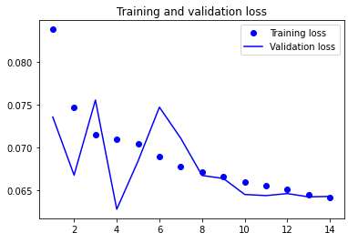
Test the model
trained_lstm_model_multi = tf.keras.models.load_model(model_path)df_temp = final_df.drop(column_name_criterium, axis=1)
test_horizon = df_temp.tail(multi_hist_window_hs)
test_history = test_horizon.values
test_scaled = scaler_x.fit_transform(test_history)
test_scaled = test_scaled.reshape(1, test_scaled.shape[0], test_scaled.shape[1])
# Inserting the model
predicted_results = trained_lstm_model_multi.predict(test_scaled)
predicted_results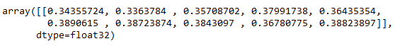
predicted_inv_trans = scaler_y.inverse_transform(predicted_results)
predicted_inv_trans
timeseries_evaluation_metrics_func(test_data[column_name_criterium], predicted_inv_trans[0])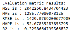
rmse_lstm_model_multi = np.sqrt(metrics.mean_squared_error(test_data[column_name_criterium], predicted_inv_trans[0]))plt.plot(list(test_data[column_name_criterium]))
plt.plot(list(predicted_inv_trans[0]))
plt.title("Actual vs Predicted")
plt.ylabel("Traffic volume")
plt.legend(('Actual','predicted'))
plt.show()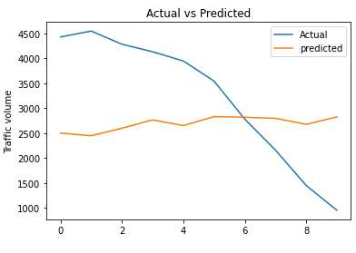
5.2 Bidirectional LSTM
Define Layer Structure
model = tf.keras.models.Sequential([
    tf.keras.layers.Bidirectional(tf.keras.layers.LSTM(150, return_sequences=True),
                                  input_shape=x_train_multi_hs.shape[-2:]),
    tf.keras.layers.Bidirectional(tf.keras.layers.LSTM(50)),
    tf.keras.layers.Dense(20, activation='tanh'),
    tf.keras.layers.Dropout(0.2),
    tf.keras.layers.Dense(units=horizon_hs)])

model.compile(loss='mse',
              optimizer='adam')
Fit the model
model_path = 'model/bi_lstm_model_multi.h5'keras_callbacks = [tf.keras.callbacks.EarlyStopping(monitor='val_loss',
min_delta=0, patience=10,
verbose=1, mode='min'),
tf.keras.callbacks.ModelCheckpoint(model_path,monitor='val_loss',
save_best_only=True,
mode='min', verbose=0)]history = model.fit(train_multi_hs, epochs=n_epochs, steps_per_epoch=n_steps_per_epoch,
validation_data=validation_multi_hs, validation_steps=n_validation_steps, verbose =1,
callbacks = keras_callbacks)Validate the model
loss = history.history['loss']
val_loss = history.history['val_loss']

epochs = range(1, len(loss) + 1)


plt.plot(epochs, loss, 'bo', label='Training loss')
plt.plot(epochs, val_loss, 'b', label='Validation loss')
plt.title('Training and validation loss')
plt.legend()

plt.show()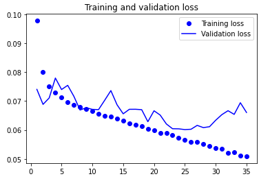
Test the model
trained_bi_lstm_model_multi = tf.keras.models.load_model(model_path)df_temp = final_df.drop(column_name_criterium, axis=1)
test_horizon = df_temp.tail(multi_hist_window_hs)
test_history = test_horizon.values
test_scaled = scaler_x.fit_transform(test_history)
test_scaled = test_scaled.reshape(1, test_scaled.shape[0], test_scaled.shape[1])
# Inserting the model
predicted_results = trained_bi_lstm_model_multi.predict(test_scaled)
predicted_results
predicted_inv_trans = scaler_y.inverse_transform(predicted_results)
predicted_inv_trans
timeseries_evaluation_metrics_func(test_data[column_name_criterium], predicted_inv_trans[0])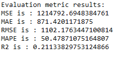
rmse_bi_lstm_model_multi = np.sqrt(metrics.mean_squared_error(test_data[column_name_criterium], predicted_inv_trans[0]))plt.plot(list(test_data[column_name_criterium]))
plt.plot(list(predicted_inv_trans[0]))
plt.title("Actual vs Predicted")
plt.ylabel("Traffic volume")
plt.legend(('Actual','predicted'))
plt.show()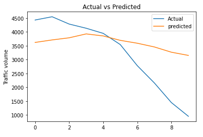
5.3 GRU
Define Layer Structure
model = tf.keras.models.Sequential([
    tf.keras.layers.GRU(100, input_shape=x_train_multi_hs.shape[-2:],return_sequences=True),
    tf.keras.layers.Dropout(0.2),
    tf.keras.layers.GRU(units=50,return_sequences=False),
    tf.keras.layers.Dropout(0.2),
    tf.keras.layers.Dense(units=horizon_hs)])

model.compile(loss='mse',
              optimizer='adam')
Fit the model
model_path = 'model/gru_model_multi.h5'keras_callbacks = [tf.keras.callbacks.EarlyStopping(monitor='val_loss',
min_delta=0, patience=10,
verbose=1, mode='min'),
tf.keras.callbacks.ModelCheckpoint(model_path,monitor='val_loss',
save_best_only=True,
mode='min', verbose=0)]history = model.fit(train_multi_hs, epochs=n_epochs, steps_per_epoch=n_steps_per_epoch,
validation_data=validation_multi_hs, validation_steps=n_validation_steps, verbose =1,
callbacks = keras_callbacks)Validate the model
loss = history.history['loss']
val_loss = history.history['val_loss']

epochs = range(1, len(loss) + 1)


plt.plot(epochs, loss, 'bo', label='Training loss')
plt.plot(epochs, val_loss, 'b', label='Validation loss')
plt.title('Training and validation loss')
plt.legend()

plt.show()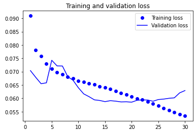
Test the model
trained_gru_model_multi = tf.keras.models.load_model(model_path)df_temp = final_df.drop(column_name_criterium, axis=1)
test_horizon = df_temp.tail(multi_hist_window_hs)
test_history = test_horizon.values
test_scaled = scaler_x.fit_transform(test_history)
test_scaled = test_scaled.reshape(1, test_scaled.shape[0], test_scaled.shape[1])
# Inserting the model
predicted_results = trained_gru_model_multi.predict(test_scaled)
predicted_results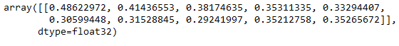
predicted_inv_trans = scaler_y.inverse_transform(predicted_results)
predicted_inv_trans
timeseries_evaluation_metrics_func(test_data[column_name_criterium], predicted_inv_trans[0])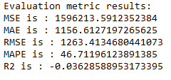
rmse_gru_model_multi = np.sqrt(metrics.mean_squared_error(test_data[column_name_criterium], predicted_inv_trans[0]))plt.plot(list(test_data[column_name_criterium]))
plt.plot(list(predicted_inv_trans[0]))
plt.title("Actual vs Predicted")
plt.ylabel("Traffic volume")
plt.legend(('Actual','predicted'))
plt.show()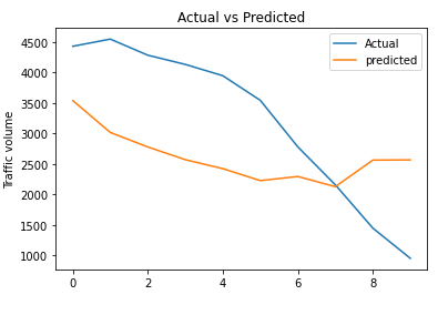
5.4 Encoder Decoder LSTM
Define Layer Structure
model = tf.keras.models.Sequential([
    tf.keras.layers.LSTM(40, input_shape=x_train_multi_hs.shape[-2:], return_sequences=True),
    tf.keras.layers.LSTM(units=20,return_sequences=True),
    tf.keras.layers.LSTM(units=15),
    tf.keras.layers.RepeatVector(y_train_multi_hs.shape[1]),
    tf.keras.layers.LSTM(units=40,return_sequences=True),
    tf.keras.layers.LSTM(units=25,return_sequences=True),
    tf.keras.layers.TimeDistributed(tf.keras.layers.Dense(units=1))])

model.compile(loss='mse',
              optimizer='adam')
Fit the model
model_path = 'model/ed_lstm_model_multi.h5'keras_callbacks = [tf.keras.callbacks.EarlyStopping(monitor='val_loss',
min_delta=0, patience=10,
verbose=1, mode='min'),
tf.keras.callbacks.ModelCheckpoint(model_path,monitor='val_loss',
save_best_only=True,
mode='min', verbose=0)]history = model.fit(train_multi_hs, epochs=n_epochs, steps_per_epoch=n_steps_per_epoch,
validation_data=validation_multi_hs, validation_steps=n_validation_steps, verbose =1,
callbacks = keras_callbacks)Validate the model
loss = history.history['loss']
val_loss = history.history['val_loss']

epochs = range(1, len(loss) + 1)


plt.plot(epochs, loss, 'bo', label='Training loss')
plt.plot(epochs, val_loss, 'b', label='Validation loss')
plt.title('Training and validation loss')
plt.legend()

plt.show()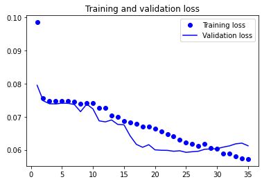
Test the model
trained_ed_lstm_model_multi = tf.keras.models.load_model(model_path)df_temp = final_df.drop(column_name_criterium, axis=1)
test_horizon = df_temp.tail(multi_hist_window_hs)
test_history = test_horizon.values
test_scaled = scaler_x.fit_transform(test_history)
test_scaled = test_scaled.reshape(1, test_scaled.shape[0], test_scaled.shape[1])
# Inserting the model
predicted_results = trained_ed_lstm_model_multi.predict(test_scaled)
predicted_results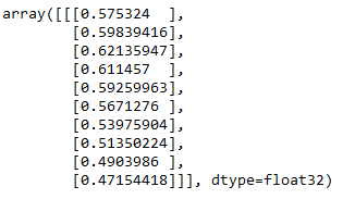
predicted_inv_trans = scaler_y.inverse_transform(predicted_results.reshape(-1,1))
predicted_inv_trans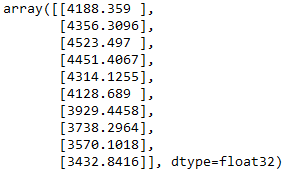
timeseries_evaluation_metrics_func(test_data[column_name_criterium], predicted_inv_trans)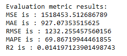
rmse_ed_lstm_model_multi = np.sqrt(metrics.mean_squared_error(test_data[column_name_criterium], predicted_inv_trans))plt.plot(list(test_data[column_name_criterium]))
plt.plot(list(predicted_inv_trans))
plt.title("Actual vs Predicted")
plt.ylabel("Traffic volume")
plt.legend(('Actual','predicted'))
plt.show()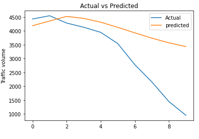
5.5 CNN
Define Layer Structure
model = tf.keras.models.Sequential()
model.add(tf.keras.layers.Conv1D(filters=64, kernel_size=3, activation='relu',
                                 input_shape=(x_train_multi_hs.shape[1], x_train_multi_hs.shape[2])))
model.add(tf.keras.layers.MaxPool1D(pool_size=2))
model.add(tf.keras.layers.Dropout(0.2))
model.add(tf.keras.layers.Flatten())
model.add(tf.keras.layers.Dense(30, activation='relu'))
model.add(tf.keras.layers.Dropout(0.2))
model.add(tf.keras.layers.Dense(units=horizon_hs))

model.compile(loss='mse',
              optimizer='adam')
Fit the model
model_path = 'model/cnn_model_multi.h5'keras_callbacks = [tf.keras.callbacks.EarlyStopping(monitor='val_loss',
min_delta=0, patience=10,
verbose=1, mode='min'),
tf.keras.callbacks.ModelCheckpoint(model_path,monitor='val_loss',
save_best_only=True,
mode='min', verbose=0)]history = model.fit(train_multi_hs, epochs=n_epochs, steps_per_epoch=n_steps_per_epoch,
validation_data=validation_multi_hs, validation_steps=n_validation_steps, verbose =1,
callbacks = keras_callbacks)Validate the model
loss = history.history['loss']
val_loss = history.history['val_loss']

epochs = range(1, len(loss) + 1)


plt.plot(epochs, loss, 'bo', label='Training loss')
plt.plot(epochs, val_loss, 'b', label='Validation loss')
plt.title('Training and validation loss')
plt.legend()

plt.show()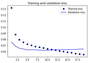
Test the model
trained_cnn_model_multi = tf.keras.models.load_model(model_path)df_temp = final_df.drop(column_name_criterium, axis=1)
test_horizon = df_temp.tail(multi_hist_window_hs)
test_history = test_horizon.values
test_scaled = scaler_x.fit_transform(test_history)
test_scaled = test_scaled.reshape(1, test_scaled.shape[0], test_scaled.shape[1])
# Inserting the model
predicted_results = trained_cnn_model_multi.predict(test_scaled)
predicted_results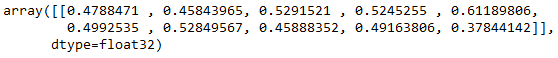
predicted_inv_trans = scaler_y.inverse_transform(predicted_results)
predicted_inv_trans
timeseries_evaluation_metrics_func(test_data[column_name_criterium], predicted_inv_trans[0])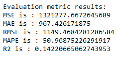
rmse_cnn_model_multi = np.sqrt(metrics.mean_squared_error(test_data[column_name_criterium], predicted_inv_trans[0]))plt.plot(list(test_data[column_name_criterium]))
plt.plot(list(predicted_inv_trans[0]))
plt.title("Actual vs Predicted")
plt.ylabel("Traffic volume")
plt.legend(('Actual','predicted'))
plt.show()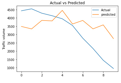
6 Get the Best Model
Let’s see which model performs best:
column_names = ["Model", "RMSE"]
df = pd.DataFrame(columns = column_names)

rmse_lstm_model_multi_df = pd.DataFrame([('lstm_model_multi', rmse_lstm_model_multi)], columns=column_names)
df = df.append(rmse_lstm_model_multi_df)

rmse_bi_lstm_model_multi_df = pd.DataFrame([('bi_lstm_model_multi', rmse_bi_lstm_model_multi)], columns=column_names)
df = df.append(rmse_bi_lstm_model_multi_df)

rmse_gru_model_multi_df = pd.DataFrame([('gru_model_multi', rmse_gru_model_multi)], columns=column_names)
df = df.append(rmse_gru_model_multi_df)

rmse_ed_lstm_model_multi_df = pd.DataFrame([('ed_lstm_model_multi', rmse_ed_lstm_model_multi)], columns=column_names)
df = df.append(rmse_ed_lstm_model_multi_df)

rmse_cnn_model_multi_df = pd.DataFrame([('cnn_model_multi', rmse_cnn_model_multi)], columns=column_names)
df = df.append(rmse_cnn_model_multi_df)

df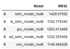
best_model = df.sort_values(by='RMSE', ascending=True)
best_model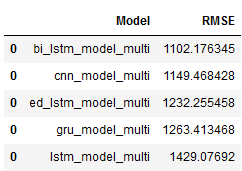
As we can see, the CNN model fits best and outperforms the other models by far.
However, it should be mentioned at this point that the neural networks created performed even better with univariate time series than with the use of multiple predictors.
7 Conclusion & Overview
In this post, I showed how to do time series analysis using neural networks with the inclusion of multiple predictors.
Looking back, I would like to give a summary of the different posts on the topic of time series analysis:
- Smoothing methods -> Prediction of 1 Target Variable over Time
- Regression Extension Techniques for Univariate Time Series -> Prediction of 1 Target Variable over Time
- Regression Extension Techniques for Multivariate Time Series -> Prediction of n Target Variable over Time
- Neural Networks for Univariate Time Series -> Prediction of 1 Target Variable over Time
- Neural Networks with multiple predictors -> Prediction of 1 Target Variable over Time with multiple predictors
References
The content of this post was inspired by:
Kaggle: Time Series Analysis using LSTM Keras from Hassan Amin
Chollet, F. (2018). Deep learning with Python (Vol. 361). New York: Manning.
Vishwas, B. V., & Patel, A. (2020). Hands-on Time Series Analysis with Python. New York: Apress. DOI: 10.1007/978-1-4842-5992-4
Medium: Time Series Forecast Using Deep Learning from Rajaram Suryanarayanan