1 Introduction

Now that I have given an introduction to the topic of time series analysis, we come to the first models with which we can make predictions for time series: Smooting Methods

The smoothing technique is a family of time-series forecasting algorithms, which utilizes the weighted averages of a previous observation to predict or forecast a new value. This technique is more efficient when time-series data is moving slowly over time. It harmonizes errors, trends and seasonal components into computing smoothing parameters.

In the following, we will look at three different smoothing methods:

Simple Exponential Smoothing
Double Exponential Smoothing
Triple Exponential Smoothing

For this post the dataset FB from the statistic platform “Kaggle” was used. You can download it from my “GitHub Repository”.

2 Import libraries and data

import pandas as pd
import numpy as np
from sklearn import metrics

import matplotlib.pyplot as plt
%matplotlib inline

from sklearn.model_selection import ParameterGrid

from statsmodels.tsa.api import SimpleExpSmoothing
from statsmodels.tsa.api import Holt
from statsmodels.tsa.api import ExponentialSmoothing

df = pd.read_csv('FB.csv')
df.head()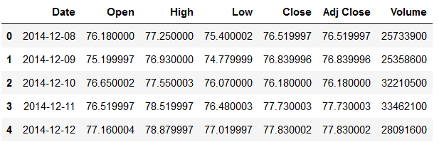

Let’s generate a training part and a test part (the last 30 values). We will focus our analysis on the ‘Close’ column. This column contains the last close of the Facebook share at the end of the respective day.

X = df['Close']

testX = X.iloc[-30:]
trainX = X.iloc[:-30]

3 Definition of required functions

For the evaluation of the following models I create a function to calculate the mean absolute percentage error and another function that outputs this metric and others for evaluation.

def mean_absolute_percentage_error_func(y_true, y_pred):
    '''
    Calculate the mean absolute percentage error as a metric for evaluation
    
    Args:
        y_true (float64): Y values for the dependent variable (test part), numpy array of floats 
        y_pred (float64): Predicted values for the dependen variable (test parrt), numpy array of floats
    
    Returns:
        Mean absolute percentage error 
    '''    
    y_true, y_pred = np.array(y_true), np.array(y_pred)
    return np.mean(np.abs((y_true - y_pred) / y_true)) * 100

def timeseries_evaluation_metrics_func(y_true, y_pred):
    '''
    Calculate the following evaluation metrics:
        - MSE
        - MAE
        - RMSE
        - MAPE
        - R²
    
    Args:
        y_true (float64): Y values for the dependent variable (test part), numpy array of floats 
        y_pred (float64): Predicted values for the dependen variable (test parrt), numpy array of floats
    
    Returns:
        MSE, MAE, RMSE, MAPE and R² 
    '''    
    print('Evaluation metric results: ')
    print(f'MSE is : {metrics.mean_squared_error(y_true, y_pred)}')
    print(f'MAE is : {metrics.mean_absolute_error(y_true, y_pred)}')
    print(f'RMSE is : {np.sqrt(metrics.mean_squared_error(y_true, y_pred))}')
    print(f'MAPE is : {mean_absolute_percentage_error_func(y_true, y_pred)}')
    print(f'R2 is : {metrics.r2_score(y_true, y_pred)}',end='\n\n')

4 Simple Exponential Smoothing

Simple Exponential Smoothing is one of the minimal models of the exponential smoothing algorithms. This method can be used to predict series that do not have trends or seasonality.

Assume that a time series has the following:

Level
No trends
No seasonality
Noise

4.1 Searching for best parameters for SES

In the Simple Exponential Smoothing function we have the following parameter that we can set:

smooting_level(float, optional)

To find out which value fits best for this we perform a for-loop.

resu = []
temp_df = pd.DataFrame()
for i in [0 , 0.10, 0.20, 0.30, 0.40, 0.50, 0.60, 0.70, 0.80, 0.90,1]:
    print(f'Fitting for smoothing level= {i}')
    fit_v = SimpleExpSmoothing(np.asarray(trainX)).fit(i)
    fcst_pred_v= fit_v.forecast(len(testX))   
    timeseries_evaluation_metrics_func(testX, fcst_pred_v)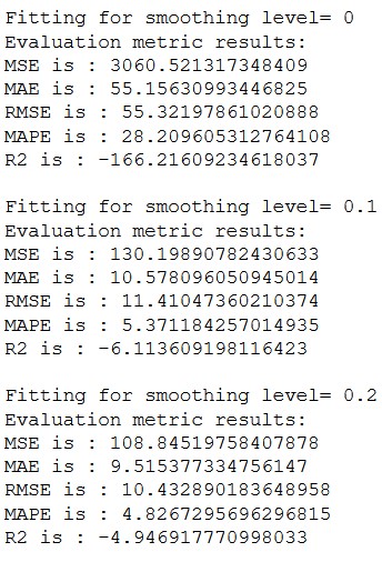

…

The output is very long and poorly comparable. So we use a for-loop to output the RMSE value for each provided smoothing parameter and store the results in a table.

resu = []
temp_df = pd.DataFrame()
for i in [0 , 0.10, 0.20, 0.30, 0.40, 0.50, 0.60, 0.70, 0.80, 0.90,1]:
    fit_v = SimpleExpSmoothing(np.asarray(trainX)).fit(i)
    fcst_pred_v= fit_v.forecast(len(testX))   
    rmse = np.sqrt(metrics.mean_squared_error(testX, fcst_pred_v))
    df3 = {'smoothing parameter':i, 'RMSE': rmse}
    temp_df = temp_df.append(df3, ignore_index=True)

temp_df.sort_values(by=['RMSE'])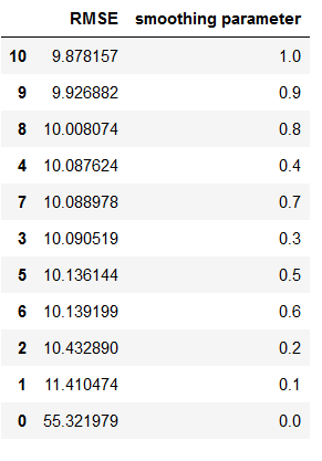

Now we can see for which smoothing parameter we get the lowest RMSE. Here: 1

4.2 Fit SES

Let’s use this value to fit our first model.

SES = SimpleExpSmoothing(np.asarray(trainX))
fit_SES = SES.fit(smoothing_level = 1, optimized=False)

fcst_gs_pred = fit_SES.forecast(len(testX))
timeseries_evaluation_metrics_func(testX, fcst_gs_pred)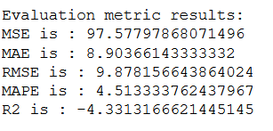

4.3 Fit SES with optimized=True

The Smoothing models also include an integrated search function for the best parameters. Let’s see if the parameters found by the algorithm itself give better results than those from our custom grid search.

SES = SimpleExpSmoothing(np.asarray(trainX))
fit_SES_auto = SES.fit(optimized= True, use_brute = True)

fcst_auto_pred = fit_SES_auto.forecast(len(testX))
timeseries_evaluation_metrics_func(testX, fcst_auto_pred)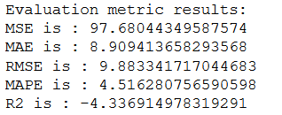

As we can see, the model with the grid serach parameters performs slightly better than the model with the self-calculated best values.

Here is an overview of which values the fit_SES_auto model has calculated:

fit_SES_auto.summary()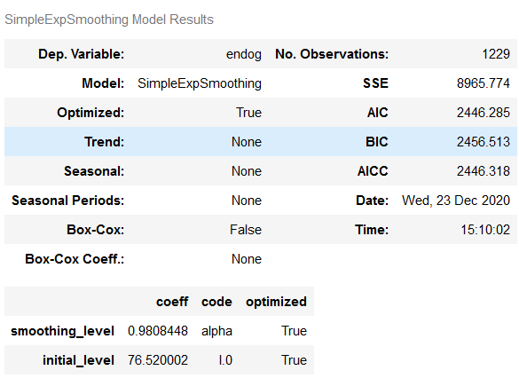

4.4 Plotting the results for SES

In order to display the results of the two calculated models nicely, we need to set the index of the predicted values equal to that of the test set.

df_fcst_gs_pred = pd.DataFrame(fcst_gs_pred, columns=['Close_grid_Search'])
df_fcst_gs_pred["new_index"] = range(len(trainX), len(X))
df_fcst_gs_pred = df_fcst_gs_pred.set_index("new_index")

df_fcst_auto_pred = pd.DataFrame(fcst_auto_pred, columns=['Close_auto_search'])
df_fcst_auto_pred["new_index"] = range(len(trainX), len(X))
df_fcst_auto_pred = df_fcst_auto_pred.set_index("new_index")

plt.rcParams["figure.figsize"] = [16,9]
plt.plot(trainX, label='Train')
plt.plot(testX, label='Test')
plt.plot(df_fcst_gs_pred, label='Simple Exponential Smoothing using custom grid search')
plt.plot(df_fcst_auto_pred, label='Simple Exponential Smoothing using optimized=True')
plt.legend(loc='best')
plt.show()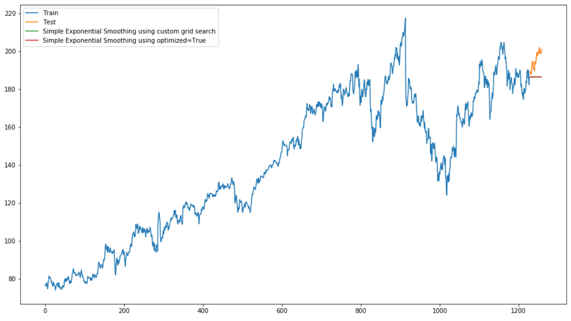

Unfortunately, in this visualization you cannot see the green and red lines that represent the predicted values for simple exponential smoothing (with grid search and optimized=True), because the two lines lie exactly on top of each other.

As we can see simple exponential smoothing does not perform very well on this data. This is because the data includes trends and seasonality.

Let’s see if it works better with other smoothing methods.

5 Double Exponential Smoothing

Let’s come to the second smooting technique: the Double Exponential Smoothing Algorithm

The Double Exponential Smoothing Algorithm is a more reliable method for handling data that consumes trends without seasonality.

Assume that a time series has the following:

Level
Trends
No seasonality
Noise

5.1 Searching for best parameters for DES

In the Double Exponential Smoothing function we have the following parameter that we can set:

damped(bool, optional)
smooting_level(float, optional)
smoothing_slope(float, optional)
damping_slope(float, optional)

To find out which value fits best for this we perform a customer grid search.

param_grid_DES = {'smoothing_level': [0.10, 0.20,.30,.40,.50,.60,.70,.80,.90], 
                  'smoothing_slope':[0.10, 0.20,.30,.40,.50,.60,.70,.80,.90],
                  'damping_slope': [0.10, 0.20,.30,.40,.50,.60,.70,.80,.90],
                  'damped': [True, False]}
pg_DES = list(ParameterGrid(param_grid_DES))

pg_DES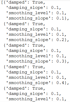

Similar to the Simple Exponential Smoothing method, we calculate the RMSE and R² for all possible parameter combinations defined within our param_grid.

df_results_DES = pd.DataFrame(columns=['smoothing_level', 'smoothing_slope', 'damping_slope', 'damped', 'RMSE','R²'])

for a,b in enumerate(pg_DES):
    smoothing_level = b.get('smoothing_level')
    smoothing_slope = b.get('smoothing_slope')
    damping_slope = b.get('damping_slope')
    damped = b.get('damped')
    
    fit_Holt = Holt(trainX, damped=damped).fit(smoothing_level=smoothing_level, smoothing_slope=smoothing_slope, damping_slope=damping_slope, optimized=False)
    fcst_gs_pred_Holt = fit_Holt.forecast(len(testX))
    
    df_pred = pd.DataFrame(fcst_gs_pred_Holt, columns=['Forecasted_result'])
    RMSE = np.sqrt(metrics.mean_squared_error(testX, df_pred.Forecasted_result))
    r2 = metrics.r2_score(testX, df_pred.Forecasted_result)

    df_results_DES = df_results_DES.append({'smoothing_level':smoothing_level, 'smoothing_slope':smoothing_slope, 'damping_slope':damping_slope, 'damped':damped, 'RMSE':RMSE, 'R²':r2}, ignore_index=True)

df_results_DES.sort_values(by=['RMSE','R²']).head(10)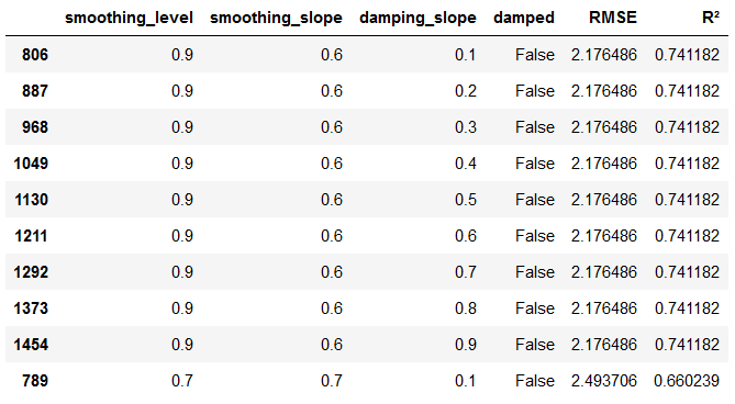

As we can see, for damped=False, smoothing_level=0.9 and smoothing_slope=0.6 we get the best RMSE and R² values. The parameter damping_slope can vary between 0.1 and 0.9, but does not influence the result. We therefore take the values from line 806.

Since such a GridSearch search can take a long time, it is recommended to save the created data set at this point.

df_results_DES.to_csv('df_results_DES.csv')

5.2 Fit DES

Let’s look at the first line of the created table with the values of our grid search. The first line tells us the best combination we can use.

best_values_DES = df_results_DES.sort_values(by=['RMSE','R²']).head(1)
best_values_DES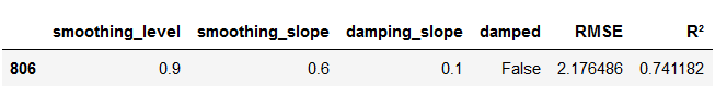

Therefore, we extract the values and insert them into our function.

smoothing_level_value_DES = best_values_DES['smoothing_level'].iloc[0]
smoothing_slope_value_DES = best_values_DES['smoothing_slope'].iloc[0]
damping_slope_value_DES = best_values_DES['damping_slope'].iloc[0]
damped_setting_DES = best_values_DES['damped'].iloc[0]

print("smoothing_level_value_DES: ", smoothing_level_value_DES)
print("smoothing_slope_value_DES: ", smoothing_slope_value_DES)
print("damping_slope_value_DES: ", damping_slope_value_DES)
print("damped_setting_DES: ", damped_setting_DES)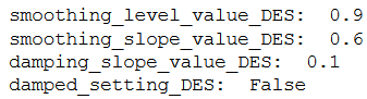

DES = Holt(trainX,damped=damped_setting_DES)
fit_Holt = DES.fit(smoothing_level=smoothing_level_value_DES, smoothing_slope=smoothing_slope_value_DES, 
                   damping_slope=damping_slope_value_DES ,optimized=False)

fcst_gs_pred_Holt = fit_Holt.forecast(len(testX))
timeseries_evaluation_metrics_func(testX, fcst_gs_pred_Holt)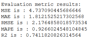

5.3 Fit DES with optimized=True

As before, let’s also output the values for an automatic search of parameters.

DES = Holt(trainX)
fit_Holt_auto = DES.fit(optimized= True, use_brute = True)

fcst_auto_pred_Holt = fit_Holt_auto.forecast(len(testX))
timeseries_evaluation_metrics_func(testX, fcst_auto_pred_Holt)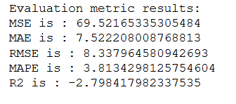

Comparing this output with the output of the first model (with grid search), we see a prime example of how the optimized=True setting can be helpful, but a more comprehensive examination of the hyperparameters with grid search can yield much better results.

fit_Holt_auto.summary()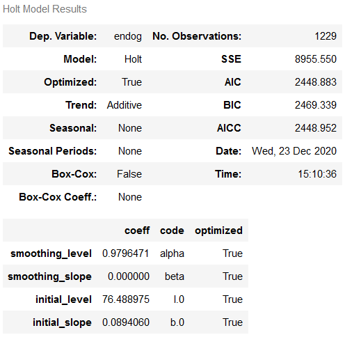

5.4 Plotting the results for DES

plt.rcParams["figure.figsize"] = [16,9]
plt.plot(trainX, label='Train')
plt.plot(testX, label='Test')
plt.plot(fcst_gs_pred_Holt, label='Double Exponential Smoothing with custom grid search')
plt.plot(fcst_auto_pred_Holt, label='Double Exponential Smoothing using optimized=True')
plt.legend(loc='best')
plt.show()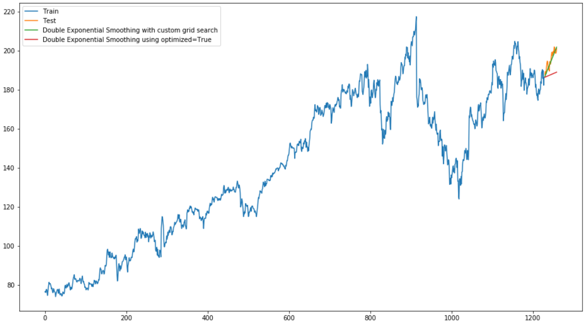

From the result, we can see that Double Exponential Smoothing works far better on this data set than Simple Exponential Smoothing.

Let’s see what values Triple Exponential Smoothing gives us.

6 Triple Exponential Smoothing

The Triple Exponential Smoothing Algorithm can be applied when the data consumes trends and seasonality over time.

Assume that a time series has the following:

Level
Trends
Seasonality
Noise

6.1 Searching for best parameters for TES

In the Double Exponential Smoothing function we have the following parameter that we can set:

trend({‘add’, ‘mul’, ‘additive’, ‘multiplicative’, None}, optional)
seasonal({‘add’, ‘mul’, ‘additive’, ‘multiplicative’, None}, optional)
seasonal_periods(int, optional)
smooting_level(float, optional)
smoothing_slope(float, optional)
damping_slope(float, optional)
damped(bool, optional)
use_boxcox({True, False, ‘log’, float}, optional)
remove_bias(bool, optional)
use_basinhopping(bool, optional)

To find out which value fits best for this we perform a customer grid search again. The procedure is known and follows the same principles as for the Double Exponential Smoothing.

param_grid_TES = {'trend': ['add', 'mul'], 'seasonal' :['add', 'mul'],
                  'seasonal_periods':[3,6,12], 
                  'smoothing_level': [.20, .40, .60, .80],  # extended search grid: [.10,.20,.30,.40,.50,.60,.70,.80,.90]
                  'smoothing_slope':[.20, .40, .60, .80],   # extended search grid: [.10,.20,.30,.40,.50,.60,.70,.80,.90]
                  'damping_slope': [.20, .40, .60, .80],    # extended search grid: [.10,.20,.30,.40,.50,.60,.70,.80,.90]
                  'damped' : [True, False], 'use_boxcox':[True, False],
                  'remove_bias':[True, False],'use_basinhopping':[True, False]}
pg_TES = list(ParameterGrid(param_grid_TES))

df_results_TES = pd.DataFrame(columns=['trend','seasonal_periods','smoothing_level', 'smoothing_slope',
                                        'damping_slope','damped','use_boxcox','remove_bias',
                                        'use_basinhopping','RMSE','R²'])

for a,b in enumerate(pg_TES):
    trend = b.get('trend')
    smoothing_level = b.get('smoothing_level')
    seasonal_periods = b.get('seasonal_periods')
    smoothing_level = b.get('smoothing_level')
    smoothing_slope = b.get('smoothing_slope')
    damping_slope = b.get('damping_slope')
    damped = b.get('damped')
    use_boxcox = b.get('use_boxcox')
    remove_bias = b.get('remove_bias')
    use_basinhopping = b.get('use_basinhopping')

    fit_ES = ExponentialSmoothing(trainX, trend=trend, damped=damped, seasonal_periods=seasonal_periods).fit(smoothing_level=smoothing_level, 
                                  smoothing_slope=smoothing_slope, damping_slope=damping_slope, use_boxcox=use_boxcox, optimized=False)
    fcst_gs_pred_ES = fit_ES.forecast(len(testX))

    df_pred = pd.DataFrame(fcst_gs_pred_ES, columns=['Forecasted_result'])
    RMSE = np.sqrt(metrics.mean_squared_error(testX, df_pred.Forecasted_result))
    r2 = metrics.r2_score(testX, df_pred.Forecasted_result)

    df_results_TES = df_results_TES.append({'trend':trend, 'seasonal_periods':seasonal_periods, 'smoothing_level':smoothing_level, 
                                            'smoothing_slope':smoothing_slope, 'damping_slope':damping_slope,'damped':damped,
                                            'use_boxcox':use_boxcox, 'remove_bias':remove_bias, 'use_basinhopping':use_basinhopping, 'RMSE':RMSE,'R²':r2}, 
                                            ignore_index=True)

df_results_TES.sort_values(by=['RMSE','R²']).head(10)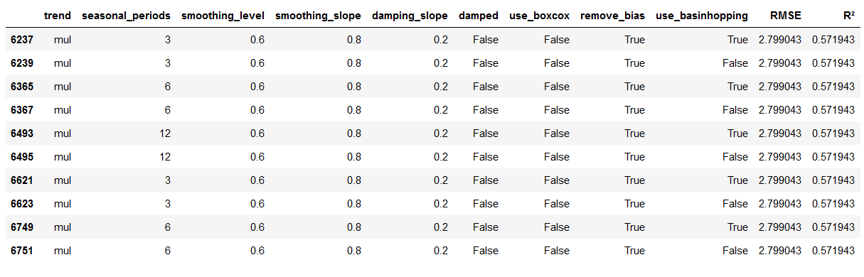

Again, we save the results dataset.

df_results_TES.to_csv('df_results_TES.csv')

6.2 Fit TES

best_values_TES = df_results_TES.sort_values(by=['RMSE','R²']).head(1)
best_values_TES

best_values_TES.info()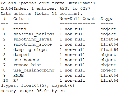

trend_setting_TES = best_values_TES['trend'].iloc[0]
damped_setting_TES = best_values_TES['damped'].iloc[0]
seasonal_periods_values_TES = best_values_TES['seasonal_periods'].iloc[0]
smoothing_level_values_TES = best_values_TES['smoothing_level'].iloc[0]
smoothing_slope_values_TES = best_values_TES['smoothing_slope'].iloc[0]
damping_slope_values_TES = best_values_TES['damping_slope'].iloc[0]
use_boxcox_setting_TES = best_values_TES['use_boxcox'].iloc[0]
remove_bias_setting_TES = best_values_TES['remove_bias'].iloc[0]     
use_basinhopping_setting_TES = best_values_TES['use_basinhopping'].iloc[0]

print("trend_setting_TES: ", trend_setting_TES)
print("damped_setting_TES: ", damped_setting_TES)
print("seasonal_periods_values_TES: ", seasonal_periods_values_TES)
print("smoothing_level_values_TES: ", smoothing_level_values_TES)
print("smoothing_slope_values_TES: ", smoothing_slope_values_TES)
print("damping_slope_values_TES: ", damping_slope_values_TES)
print("use_boxcox_setting_TES: ", use_boxcox_setting_TES)
print("remove_bias_setting_TES: ", remove_bias_setting_TES)
print("use_basinhopping_setting_TES: ", use_basinhopping_setting_TES)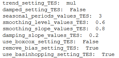

TES = ExponentialSmoothing(trainX, trend=trend_setting_TES, damped=damped_setting_TES, 
                           seasonal_periods=seasonal_periods_values_TES)
fit_ES = TES.fit(smoothing_level=smoothing_level_values_TES, smoothing_slope=smoothing_slope_values_TES, 
                 damping_slope=damping_slope_values_TES, use_boxcox=use_boxcox_setting_TES, 
                 remove_bias=remove_bias_setting_TES, optimized=False)

fcst_gs_pred_ES = fit_ES.forecast(len(testX))
timeseries_evaluation_metrics_func(testX, fcst_gs_pred_ES)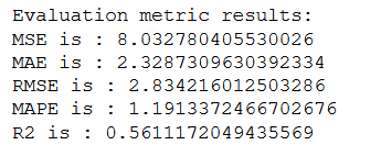

6.3 Fit TES with optimized=True

TES = ExponentialSmoothing(trainX)
fit_ES_auto = TES.fit(optimized= True, use_brute = True)

fcst_auto_pred_ES = fit_ES_auto.forecast(len(testX))
timeseries_evaluation_metrics_func(testX, fcst_auto_pred_ES)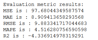

Once again, the model with the values from grid search delivers the better results.

fit_ES_auto.summary()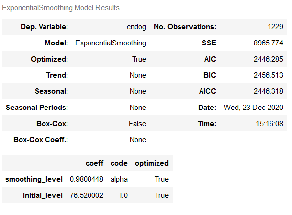

6.4 Plotting the results for TES

plt.rcParams["figure.figsize"] = [16,9]
plt.plot(trainX, label='Train')
plt.plot(testX, label='Test')
plt.plot(fcst_gs_pred_ES, label='Triple Exponential Smoothing with custom grid search')
plt.plot(fcst_auto_pred_ES, label='Triple Exponential Smoothing using optimized=True')
plt.legend(loc='best')
plt.show()

This model also scores well. But overall, the Double Exponential Smoothing model performs best.

7 Conclusion

In this post I presented the first algorithms with which you can make time series predictions.

References

The content of the entire post was created using the following sources:

Vishwas, B. V., & Patel, A. (2020). Hands-on Time Series Analysis with Python. New York: Apress. DOI: 10.1007/978-1-4842-5992-4

Time Series Analysis - Smoothing Methods

1 Introduction

2 Import libraries and data

3 Definition of required functions

4 Simple Exponential Smoothing

4.1 Searching for best parameters for SES

4.2 Fit SES

4.3 Fit SES with optimized=True

4.4 Plotting the results for SES

5 Double Exponential Smoothing

5.1 Searching for best parameters for DES

5.2 Fit DES

5.3 Fit DES with optimized=True

5.4 Plotting the results for DES

6 Triple Exponential Smoothing

6.1 Searching for best parameters for TES

6.2 Fit TES

6.3 Fit TES with optimized=True

6.4 Plotting the results for TES

7 Conclusion