1 Introduction
2 Theoretical Background
3 Import the Libraries and Data
4 Definition of required Functions
5 Check for Stationarity
6 ARIMA in Action
7 Seasonal ARIMA (SARIMA)
- 7.1 Get the final Model
8 SARIMAX
- 8.1 Get the final Model
9 Conclusion

1 Introduction

Now that we are familiar with smoothing methods for predicting time series, we come to so-called regression extension techniques.

Univariate vs. Multivariate Time Series

Since these terms often cause confusion, I would like to explain these differences again at the beginning.

Univariate

This post will be about Univariate Time Series Analysis. This means we look at the time course of only one variable and try to build a model to predict future values based on the past course.

Multivariate

The following post I plan to write is about Multivariate Time Series Analysis. In this case, several dependent/target variables (criterions) are considered simultaneously and values for them are predicted. This is not to be confused with multiple models. Here, several independent variables (predictors) are used to explain a dependent variable.

Overview of the algorithms used

In the following I will present the following algorithms:

ARIMA
SARIMA
SARIMAX

For this post the dataset FB from the statistic platform “Kaggle” was used. You can download it from my “GitHub Repository”.

2 Theoretical Background

Before we jump in with Regression Extension Techniques, it is worthwhile to understand some theoretical terminology and what it means for the algorithms that follow.

Autoregressive Models

In an autoregression model, we forecast the variable of interest using a linear combination of past values of the variable. The term autoregression indicates that it is a regression of the variable against itself.

Autocorrelation

Autocorrelation refers to the degree of correlation between the values of the same variables across different observations in the data. After checking the ACF helps in determining if differencing is required or not.

Moving Average

A moving average (MA) is a calculation used to analyze data points by creating a series of averages of different subsets of the full data set. It is utilized for long-term forecasting trends.

The Integration (I)

Time-series data is often nonstationary and to make them stationary, the series needs to be differentiated. This process is known as the integration part (I), and the order of differencing is signified as d.

Autoregressive Integrated Moving Average

Autoregressive Integrated Moving Average - also called ARIMA(p,d,q) is a forecasting equation that can make time series stationary and thus predict future trends.

ARIMA is a method among several used for forecasting univariate variables and has three components: the autoregression part (AR), the integration part (I) and the moving average part (MA).

ARIMA is made up of two models: AR and MA

3 Import the Libraries and Data

import numpy as np
import pandas as pd

import matplotlib.pyplot as plt
%matplotlib inline
from statsmodels.tsa.stattools import adfuller
from sklearn import metrics
import matplotlib.pyplot as plt
%matplotlib inline

from pmdarima import auto_arima
from pmdarima.model_selection import train_test_split as time_train_test_split

df = pd.read_csv('FB.csv')
df.head()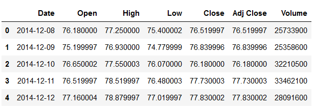

Let’s have a closer look at the target column ‘Close’:

df["Close"].plot(figsize=(15, 6))
plt.xlabel("Date")
plt.ylabel("Close")
plt.title("Closing price of Facebook stocks from 2014 to 2019")
plt.show()

plt.figure(1, figsize=(15,6))
plt.subplot(211)
df["Close"].hist()
plt.subplot(212)
df["Close"].plot(kind='kde')
plt.show()

4 Definition of required Functions

def mean_absolute_percentage_error_func(y_true, y_pred):
    '''
    Calculate the mean absolute percentage error as a metric for evaluation
    
    Args:
        y_true (float64): Y values for the dependent variable (test part), numpy array of floats 
        y_pred (float64): Predicted values for the dependen variable (test parrt), numpy array of floats
    
    Returns:
        Mean absolute percentage error 
    '''    
    y_true, y_pred = np.array(y_true), np.array(y_pred)
    return np.mean(np.abs((y_true - y_pred) / y_true)) * 100

def timeseries_evaluation_metrics_func(y_true, y_pred):
    '''
    Calculate the following evaluation metrics:
        - MSE
        - MAE
        - RMSE
        - MAPE
        - R²
    
    Args:
        y_true (float64): Y values for the dependent variable (test part), numpy array of floats 
        y_pred (float64): Predicted values for the dependen variable (test parrt), numpy array of floats
    
    Returns:
        MSE, MAE, RMSE, MAPE and R² 
    '''    
    print('Evaluation metric results: ')
    print(f'MSE is : {metrics.mean_squared_error(y_true, y_pred)}')
    print(f'MAE is : {metrics.mean_absolute_error(y_true, y_pred)}')
    print(f'RMSE is : {np.sqrt(metrics.mean_squared_error(y_true, y_pred))}')
    print(f'MAPE is : {mean_absolute_percentage_error_func(y_true, y_pred)}')
    print(f'R2 is : {metrics.r2_score(y_true, y_pred)}',end='\n\n')

def Augmented_Dickey_Fuller_Test_func(timeseries , column_name):
    '''
    Calculates statistical values whether the available data are stationary or not 
    
    Args:
        series (float64): Values of the column for which stationarity is to be checked, numpy array of floats 
        column_name (str): Name of the column for which stationarity is to be checked
    
    Returns:
        p-value that indicates whether the data are stationary or not
    ''' 
    print (f'Results of Dickey-Fuller Test for column: {column_name}')
    adfTest = adfuller(timeseries, autolag='AIC')
    dfResults = pd.Series(adfTest[0:4], index=['ADF Test Statistic','P-Value','# Lags Used','# Observations Used'])
    for key, value in adfTest[4].items():
       dfResults['Critical Value (%s)'%key] = value
    print (dfResults)
    if adfTest[1] <= 0.05:
        print()
        print("Conclusion:")
        print("Reject the null hypothesis")
        print('\033[92m' + "Data is stationary" + '\033[0m')
    else:
        print()
        print("Conclusion:")
        print("Fail to reject the null hypothesis")
        print('\033[91m' + "Data is non-stationary" + '\033[0m')

5 Check for Stationarity

Augmented_Dickey_Fuller_Test_func(df['Close' ],'Close')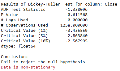

As we can see from the result, the present time series is not stationary.

However, Auto_arima can handle this internally!

Therefore, it is not necessary at this point to differentiate the data as I have done, for example, in the following post: Multivariate Time Series - Make data stationary

6 ARIMA in Action

X = df['Close']

trainX, testX = time_train_test_split(X, test_size=30)

The pmdarima modul will help us identify p,d and q without the hassle of looking at the plot. For a simple ARIMA model we have to use seasonal=False.

stepwise_model = auto_arima(trainX,start_p=1, start_q=1,
                            max_p=7, max_q=7, seasonal = False,
                            d=None, trace=True,error_action='ignore',
                            suppress_warnings=True, stepwise=True)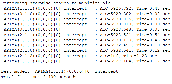

Now we are going to forecast both results and the confidence for the next 30 days.

forecast, conf_int = stepwise_model.predict(n_periods=len(testX), return_conf_int=True)

forecast = pd.DataFrame(forecast,columns=['close_pred'])

Here we store the values of the confidence within a dataframe.

df_conf = pd.DataFrame(conf_int,columns= ['Upper_bound','Lower_bound'])
df_conf["new_index"] = range(len(trainX), len(X))
df_conf = df_conf.set_index("new_index")

df_conf.head()

timeseries_evaluation_metrics_func(testX, forecast)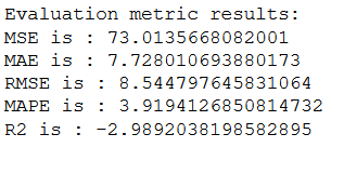

To visualize the results nicely we need to assign the appropriate index to the predicted values.

forecast["new_index"] = range(len(trainX), len(X))
forecast = forecast.set_index("new_index")

plt.rcParams["figure.figsize"] = [15,7]
plt.plot(trainX, label='Train ')
plt.plot(testX, label='Test ')
plt.plot(forecast, label='Predicted ')
plt.plot(df_conf['Upper_bound'], label='Confidence Interval Upper bound ')
plt.plot(df_conf['Lower_bound'], label='Confidence Interval Lower bound ')
plt.legend(loc='best')
plt.show()

We are also able to visualize a diagnostic plot:

stepwise_model.plot_diagnostics()

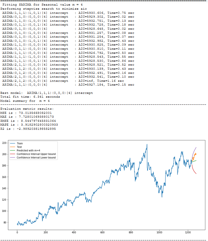
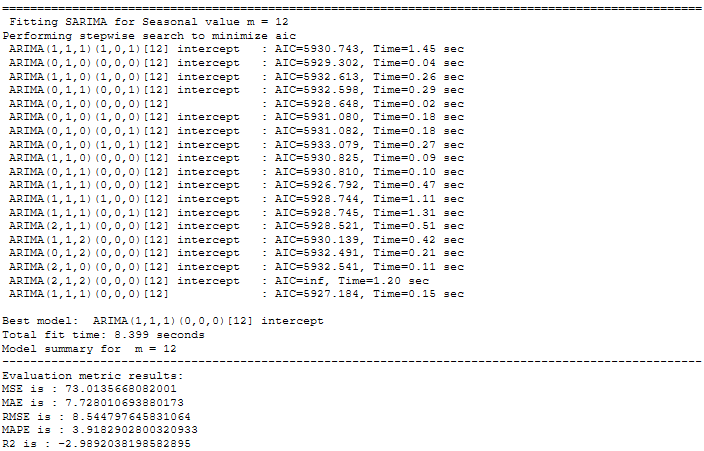
7 Seasonal ARIMA (SARIMA)

Seasonal ARIMA (SARIMA) is a technique of ARIMA, where the seasonal component can be handled in univariate time-series data.

df_results_SARIMA = pd.DataFrame()


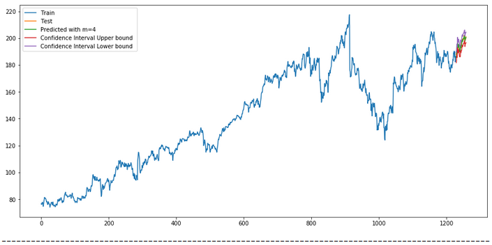
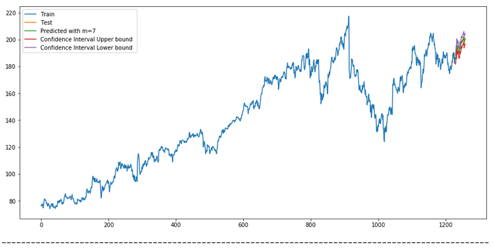
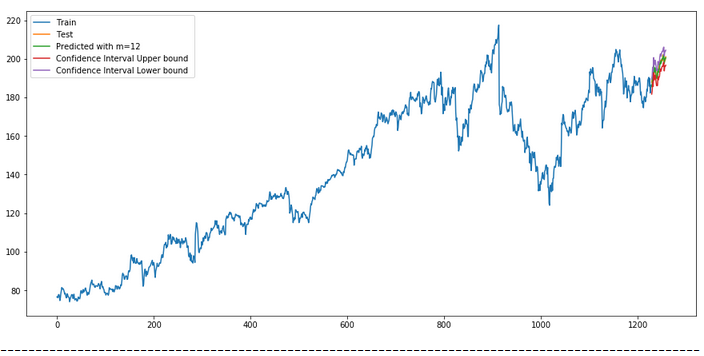
for m in  [1, 4, 7, 12, 52]:
    print("="*100)
    print(f' Fitting SARIMA for Seasonal value m = {str(m)}')
    stepwise_model = auto_arima(trainX, start_p=1, start_q=1,
                                max_p=7, max_q=7, seasonal=True, start_P=1, 
                                start_Q=1, max_P=7, max_D=7, max_Q=7, m=m,
                                d=None, D=None, trace=True, error_action='ignore', 
                                suppress_warnings=True, stepwise=True)

    print(f'Model summary for  m = {str(m)}')
    print("-"*100)
    stepwise_model.summary()

    forecast ,conf_int= stepwise_model.predict(n_periods=len(testX),return_conf_int=True)
    df_conf = pd.DataFrame(conf_int,columns= ['Upper_bound','Lower_bound'])
    df_conf["new_index"] = range(len(trainX), len(X))
    df_conf = df_conf.set_index("new_index")
    forecast = pd.DataFrame(forecast, columns=['close_pred'])
    forecast["new_index"] = range(len(trainX), len(X))
    forecast = forecast.set_index("new_index")

    timeseries_evaluation_metrics_func(testX, forecast)
    
    
    # Storage of m value for each model in a separate table 
    rmse = np.sqrt(metrics.mean_squared_error(testX, forecast))    
    df1 = {'m':m, 'RMSE': rmse}
    df_results_SARIMA = df_results_SARIMA.append(df1, ignore_index=True)

    
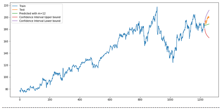
    plt.rcParams["figure.figsize"] = [15, 7]
    plt.plot(trainX, label='Train ')
    plt.plot(testX, label='Test ')
    plt.plot(forecast, label=f'Predicted with m={str(m)} ')
    plt.plot(df_conf['Upper_bound'], label='Confidence Interval Upper bound ')
    plt.plot(df_conf['Lower_bound'], label='Confidence Interval Lower bound ')
    plt.legend(loc='best')
    plt.show()
    
    print("-"*100)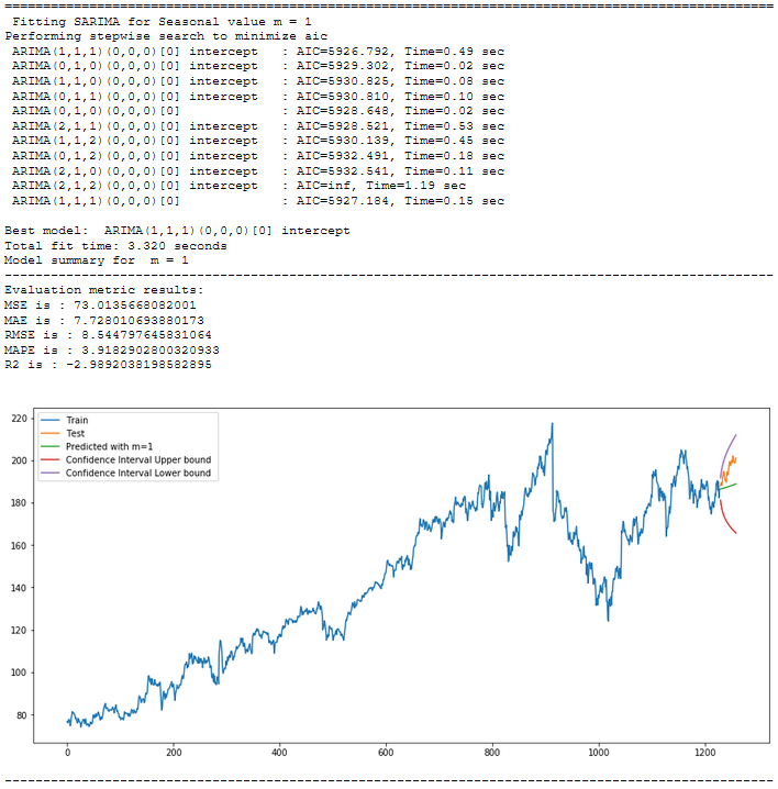

7.1 Get the final Model

df_results_SARIMA.sort_values(by=['RMSE'])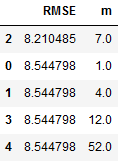

best_values_SARIMA = df_results_SARIMA.sort_values(by=['RMSE']).head(1)
best_values_SARIMA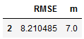

m_value_SARIMA = best_values_SARIMA['m'].iloc[0]

print("m_value_SARIMA: ", m_value_SARIMA)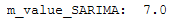

With the for-loop we have now found out for which value m we get the best results. This was the case for m=7. Now we execute auto_arima again with m=7 to have the best values stored in the stepwise_model and to be able to apply this model.

stepwise_model = auto_arima(trainX, start_p=1, start_q=1, max_p=7, max_q=7, seasonal=True, 
                            start_P=1, start_Q=1, max_P=7, max_D=7, max_Q=7, m=int(m_value_SARIMA),
                            d=None, D=None, trace=True, error_action='ignore', 
                            suppress_warnings=True, stepwise=True)

forecast, conf_int = stepwise_model.predict(n_periods=len(testX), return_conf_int=True)
forecast = pd.DataFrame(forecast,columns=['close_pred'])

timeseries_evaluation_metrics_func(testX, forecast)

df_conf = pd.DataFrame(conf_int,columns= ['Upper_bound','Lower_bound'])
df_conf["new_index"] = range(len(trainX), len(X))
df_conf = df_conf.set_index("new_index")

forecast["new_index"] = range(len(trainX), len(X))
forecast = forecast.set_index("new_index")

plt.rcParams["figure.figsize"] = [15,7]
plt.plot(trainX, label='Train ')
plt.plot(testX, label='Test ')
plt.plot(forecast, label='Predicted ')
plt.plot(df_conf['Upper_bound'], label='Confidence Interval Upper bound ')
plt.plot(df_conf['Lower_bound'], label='Confidence Interval Lower bound ')
plt.legend(loc='best')
plt.show()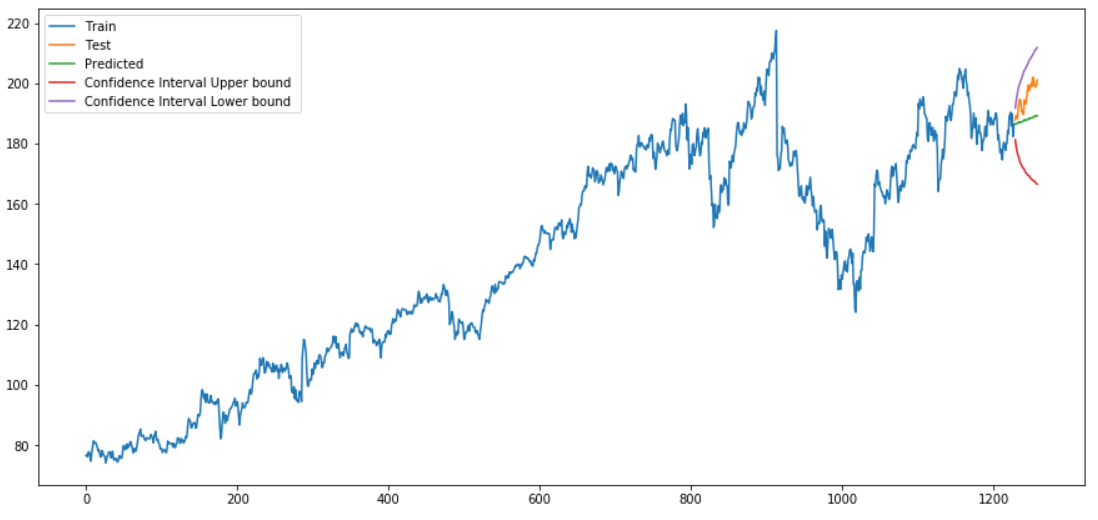

8 SARIMAX

The SARIMAX model is a SARIMA model with external influencing variables.

We know from the column ‘Close’ that it is non-stationary. But what about the other columns?

for name, column in df[['Close' ,'Open' ,'High','Low']].iteritems():
    Augmented_Dickey_Fuller_Test_func(df[name],name)
    print('\n')

Like ARIMA, SARIMAX can handle non-stationary time series internally as well.

In the following, modeling will be done only for the column ‘Close’. The column ‘Open’ will be used as exogenous variables.

X = df[['Close']]

actualtrain, actualtest = time_train_test_split(X, test_size=30)

exoX = df[['Open']]

exotrain, exotest = time_train_test_split(exoX, test_size=30)

Let’s configure and run seasonal ARIMA with an exogenous variable.

df_results_SARIMAX = pd.DataFrame()

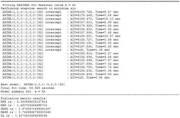
for m in [1, 4, 7, 12, 52]:
    print("="*100)
    print(f' Fitting SARIMAX for Seasonal value m = {str(m)}')
    stepwise_model = auto_arima(actualtrain,exogenous=exotrain ,start_p=1, start_q=1,
    max_p=7, max_q=7, seasonal=True,start_P=1,start_Q=1,max_P=7,max_D=7,max_Q=7,m=m,
    d=None,D=None, trace=True,error_action='ignore',suppress_warnings=True, stepwise=True)

    print(f'Model summary for  m = {str(m)}')
    print("-"*100)
    stepwise_model.summary()

    forecast,conf_int = stepwise_model.predict(n_periods=len(actualtest),
                                               exogenous=exotest,return_conf_int=True)
    df_conf = pd.DataFrame(conf_int,columns= ['Upper_bound','Lower_bound'])
    df_conf["new_index"] = range(len(actualtrain), len(X))
    df_conf = df_conf.set_index("new_index")
    forecast = pd.DataFrame(forecast, columns=['close_pred'])
    forecast["new_index"] = range(len(actualtrain), len(X))
    forecast = forecast.set_index("new_index")

    timeseries_evaluation_metrics_func(actualtest, forecast)

    # Storage of m value for each model in a separate table 
    rmse = np.sqrt(metrics.mean_squared_error(actualtest, forecast))    
    df1 = {'m':m, 'RMSE': rmse}
    df_results_SARIMAX = df_results_SARIMAX.append(df1, ignore_index=True)
    
    
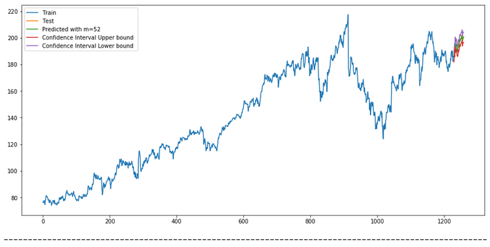
    plt.rcParams["figure.figsize"] = [15, 7]
    plt.plot(actualtrain, label='Train')
    plt.plot(actualtest, label='Test')
    plt.plot(forecast, label=f'Predicted with m={str(m)} ')
    plt.plot(df_conf['Upper_bound'], label='Confidence Interval Upper bound ')
    plt.plot(df_conf['Lower_bound'], label='Confidence Interval Lower bound ')
    plt.legend(loc='best')
    plt.show()

    print("-"*100)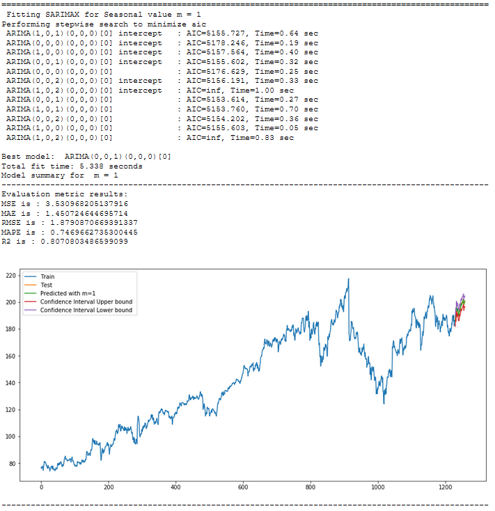

8.1 Get the final Model

Again, we have the RMSE values stored in a separate table.

df_results_SARIMAX.sort_values(by=['RMSE'])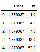

Let’s have a look at the first row (which shows the best RMSE value).

best_values_SARIMAX = df_results_SARIMAX.sort_values(by=['RMSE']).head(1)
best_values_SARIMAX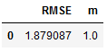

Now we are going to extract the m value for our final model.

m_value_SARIMAX = best_values_SARIMAX['m'].iloc[0]

print("m_value_SARIMAX: ", m_value_SARIMAX)

stepwise_model = auto_arima(actualtrain,exogenous=exotrain ,start_p=1, start_q=1,
    max_p=7, max_q=7, seasonal=True,start_P=1,start_Q=1,max_P=7,max_D=7,max_Q=7,m=int(m_value_SARIMAX),
    d=None,D=None, trace=True,error_action='ignore',suppress_warnings=True, stepwise=True)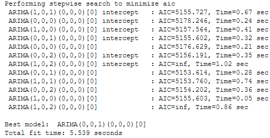

forecast,conf_int = stepwise_model.predict(n_periods=len(actualtest),
                                            exogenous=exotest,return_conf_int=True)
    
forecast = pd.DataFrame(forecast, columns=['close_pred'])

timeseries_evaluation_metrics_func(actualtest, forecast)

df_conf = pd.DataFrame(conf_int,columns= ['Upper_bound','Lower_bound'])
df_conf["new_index"] = range(len(actualtrain), len(X))
df_conf = df_conf.set_index("new_index")

forecast["new_index"] = range(len(actualtrain), len(X))
forecast = forecast.set_index("new_index")

plt.rcParams["figure.figsize"] = [15, 7]
plt.plot(actualtrain, label='Train')
plt.plot(actualtest, label='Test')
plt.plot(forecast, label=f'Predicted')
plt.plot(df_conf['Upper_bound'], label='Confidence Interval Upper bound ')
plt.plot(df_conf['Lower_bound'], label='Confidence Interval Lower bound ')
plt.legend(loc='best')
plt.show()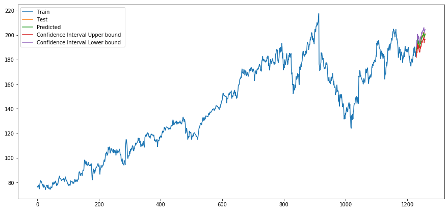

9 Conclusion

In this post, I started with a theoretical overview of the most important issues surrounding time series prediction algorithms.

Furthermore, I presented the following algorithms:

ARIMA
SARIMA
SARIMAX

These were used to predict values for univariate time series. In my following post I will present algorithms that allow the prediction of multiple target variables.

References

The content of this post was inspired by:

Machine Learning Plus: Time Series Analysis in Python – A Comprehensive Guide with Examples from Selva Prabhakaran

Kaggle: Complete Guide on Time Series Analysis in Python from Prashant Banerjee

Vishwas, B. V., & Patel, A. (2020). Hands-on Time Series Analysis with Python. New York: Apress. DOI: 10.1007/978-1-4842-5992-4

Medium: A Brief Introduction to ARIMA and SARIMAX Modeling in Python from Datascience George