1 Introduction
In my last post (“Regression Extension Techniques for Univariate Time Series”) I showed how to make time series predictions of single variables. Now we come to the exciting topic of how to do this for multiple target variables at the same time.
For this post the dataset FB from the statistic platform “Kaggle” was used. You can download it from my “GitHub Repository”.
2 Import the Libraries and the Data
import numpy as np
import pandas as pd

import matplotlib.pyplot as plt
%matplotlib inline

# Libraries to define the required functions
from statsmodels.tsa.stattools import adfuller
from statsmodels.tsa.vector_ar.vecm import coint_johansen

from pmdarima.model_selection import train_test_split as time_train_test_split
from sklearn import metrics
from sklearn.model_selection import ParameterGrid

from statsmodels.tsa.api import VAR
from statsmodels.tsa.statespace.varmax import VARMAX
from pmdarima import auto_arima


import warnings
warnings.filterwarnings("ignore")
df = pd.read_csv('FB.csv')
df.head()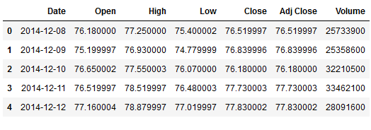
3 Definition of required Functions
def mean_absolute_percentage_error_func(y_true, y_pred):
    '''
    Calculate the mean absolute percentage error as a metric for evaluation

    Args:
        y_true (float64): Y values for the dependent variable (test part), numpy array of floats
        y_pred (float64): Predicted values for the dependen variable (test parrt), numpy array of floats

    Returns:
        Mean absolute percentage error
    '''
    y_true, y_pred = np.array(y_true), np.array(y_pred)
    return np.mean(np.abs((y_true - y_pred) / y_true)) * 100
def timeseries_evaluation_metrics_func(y_true, y_pred):
'''
Calculate the following evaluation metrics:
- MSE
- MAE
- RMSE
- MAPE
- R²
Args:
y_true (float64): Y values for the dependent variable (test part), numpy array of floats
y_pred (float64): Predicted values for the dependen variable (test parrt), numpy array of floats
Returns:
MSE, MAE, RMSE, MAPE and R²
'''
print('Evaluation metric results: ')
print(f'MSE is : {metrics.mean_squared_error(y_true, y_pred)}')
print(f'MAE is : {metrics.mean_absolute_error(y_true, y_pred)}')
print(f'RMSE is : {np.sqrt(metrics.mean_squared_error(y_true, y_pred))}')
print(f'MAPE is : {mean_absolute_percentage_error_func(y_true, y_pred)}')
print(f'R2 is : {metrics.r2_score(y_true, y_pred)}',end='\n\n')def Augmented_Dickey_Fuller_Test_func(timeseries , column_name):
'''
Calculates statistical values whether the available data are stationary or not
Args:
series (float64): Values of the column for which stationarity is to be checked, numpy array of floats
column_name (str): Name of the column for which stationarity is to be checked
Returns:
p-value that indicates whether the data are stationary or not
'''
print (f'Results of Dickey-Fuller Test for column: {column_name}')
adfTest = adfuller(timeseries, autolag='AIC')
dfResults = pd.Series(adfTest[0:4], index=['ADF Test Statistic','P-Value','# Lags Used','# Observations Used'])
for key, value in adfTest[4].items():
dfResults['Critical Value (%s)'%key] = value
print (dfResults)
if adfTest[1] <= 0.05:
print()
print("Conclusion:")
print("Reject the null hypothesis")
print('\033[92m' + "Data is stationary" + '\033[0m')
else:
print()
print("Conclusion:")
print("Fail to reject the null hypothesis")
print('\033[91m' + "Data is non-stationary" + '\033[0m')def cointegration_test_func(df):
'''
Test if there is a long-run relationship between features
Args:
dataframe (float64): Values of the columns to be checked, numpy array of floats
Returns:
True or False whether a variable has a long-run relationship between other features
'''
johansen_cointegration_test = coint_johansen(df,-1,5)
c = {'0.90':0, '0.95':1, '0.99':2}
traces = johansen_cointegration_test.lr1
cvts = johansen_cointegration_test.cvt[:, c[str(1-0.05)]]
def adjust(val, length= 6):
return str(val).ljust(length)
print('Column_Name > Test_Stat > C(95%) => Signif \n', '--'*25)
for col, trace, cvt in zip(df.columns, traces, cvts):
print(adjust(col), ' > ',
adjust(round(trace,2), 9), " > ",
adjust(cvt, 8), ' => ' ,
trace > cvt)def inverse_diff_func(actual_df, pred_df):
'''
Transforms the differentiated values back
Args:
actual dataframe (float64): Values of the columns, numpy array of floats
predicted dataframe (float64): Values of the columns, numpy array of floats
Returns:
Dataframe with the predicted values
'''
df_temp = pred_df.copy()
columns = actual_df.columns
for col in columns:
df_temp[str(col)+'_inv_diff'] = actual_df[col].iloc[-1] + df_temp[str(col)].cumsum()
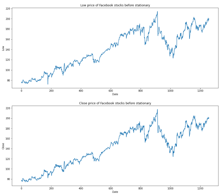
return df_temp4 EDA
for feature in df[['Open', 'High', 'Low', 'Close']]:
    df[str(feature)].plot(figsize=(15, 6))
    plt.xlabel("Date")
    plt.ylabel(feature)
    plt.title(f"{str(feature)} price of Facebook stocks before stationary")
    plt.show()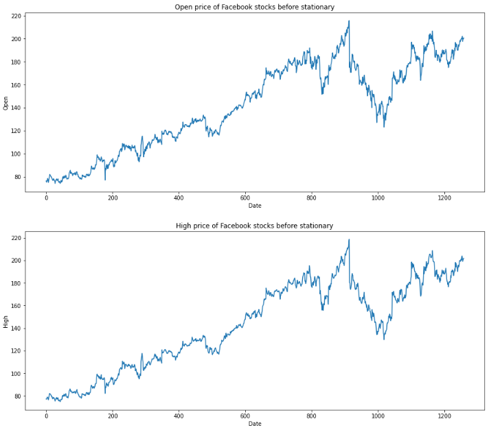
5 Stationarity
5.1 Check for stationary
for name, column in df[['Open', 'High', 'Low', 'Close']].iteritems():
    Augmented_Dickey_Fuller_Test_func(df[name],name)
    print('\n')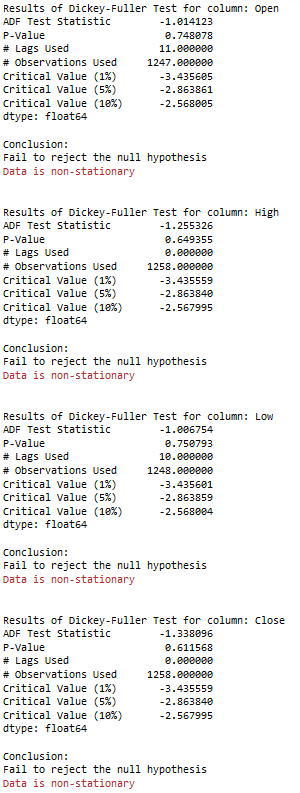
5.2 Train Test Split
X = df[['Open', 'High', 'Low', 'Close' ]]

trainX, testX = time_train_test_split(X, test_size=30)
5.3 Make data stationary
train_diff = trainX.diff()
train_diff.dropna(inplace = True)
5.4 Check again for stationary
for name, column in train_diff.iteritems():
    Augmented_Dickey_Fuller_Test_func(train_diff[name],name)
    print('\n')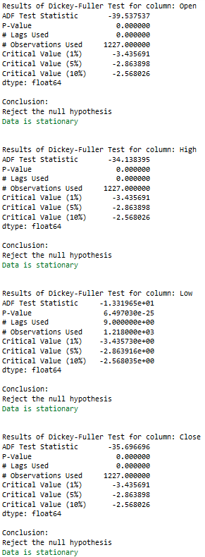
6 Cointegration Test
A cointegration test is the co-movement among underlying variables over the long run. This long-run estimation feature distinguishes it from correlation. Two or more variables are cointegrated if ond only if they share common trends.
In comparison: The Correlation is simply a measure of the degree of mutual association between two or more variables.
cointegration_test_func(train_diff)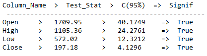
As we can see from the output, there is the presence of a long-run relationship between features.
7 Regression Extension Techniques for Forecasting Multivariate Variables
7.1 Vector Autoregression (VAR)
Vector Autoregression (VAR) is a stochastic process model utilized to seize the linear relation among the multiple variables of time-series data. VAR is a bidirectional model, while others are undirectional. In a undirectionla model, a predictor influences the target variable, but not vice versa. In a bidirectional model, variables influence each other.
7.1.1 Get best AR Terms
First of all we fit the VAR model wth AR terms between 1 to 9 and choose the best AR component.
resu = []
df_results_VAR = pd.DataFrame()

for i in [1,2,3,4,5,6,7,8,9]:
    fit_v = VAR(train_diff).fit(i)
    aic = fit_v.aic
    bic = fit_v.bic
    df1 = {'AR_Term':i, 'AIC': aic, 'BIC': bic}
    df_results_VAR = df_results_VAR.append(df1, ignore_index=True)
    clist = ['AR_Term','AIC','BIC']
    df_results_VAR = df_results_VAR[clist]
df_results_VAR.sort_values(by=['AIC', 'BIC'], ascending=True)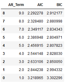
best_values_VAR = df_results_VAR.sort_values(by=['AIC', 'BIC']).head(1)
best_values_VAR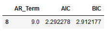
AR_Term_value_VAR = best_values_VAR['AR_Term'].iloc[0]

print("AR_Term_value_VAR: ", AR_Term_value_VAR)
Autoregressive AR(9) appears to be providing the least AIC.
7.1.2 Fit VAR
model = VAR(train_diff).fit(int(AR_Term_value_VAR))

result = model.forecast(y=train_diff.values, steps=len(testX))
7.1.3 Inverse Transformation
df_pred = pd.DataFrame(result, columns=train_diff.columns)
df_pred["new_index"] = range(len(trainX), len(X))
df_pred = df_pred.set_index("new_index")
df_pred.head()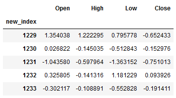
res = inverse_diff_func(trainX, df_pred)
res.head()
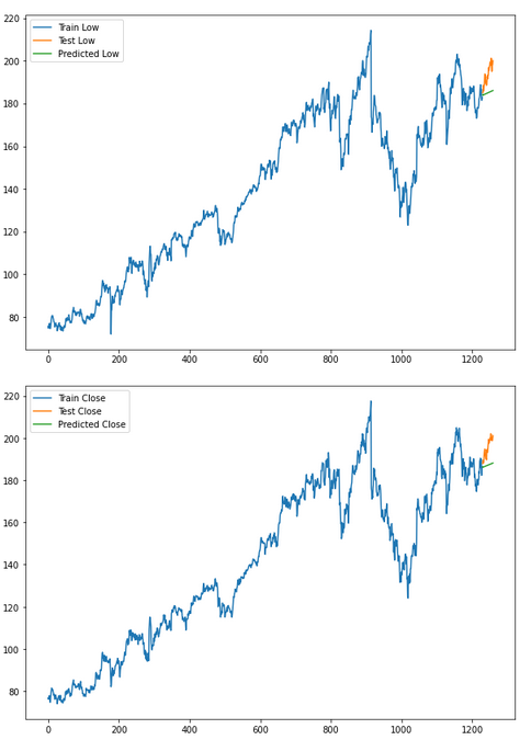
7.1.4 Evaluation of VAR
for i in ['Open', 'High', 'Low', 'Close' ]:
    print(f'Evaluation metric for {i}')
    timeseries_evaluation_metrics_func(testX[str(i)] , res[str(i)+'_inv_diff'])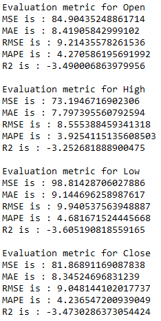
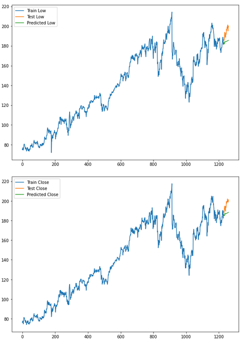
for i in ['Open', 'High', 'Low', 'Close' ]:

    plt.rcParams["figure.figsize"] = [10,7]
    plt.plot(trainX[str(i)], label='Train '+str(i))
    plt.plot(testX[str(i)], label='Test '+str(i))
    plt.plot(res[str(i)+'_inv_diff'], label='Predicted '+str(i))
    plt.legend(loc='best')
    plt.show()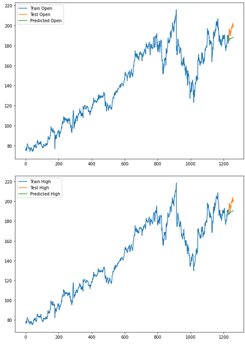
7.2 VARMA
A VARMA model is another extension of the ARMA model for a multivariate time-series model that contains a vector autoregressive (VAR) component, as well as the vector moving average (VMA). The method is used for multivariate time-series data deprived of trend and seasonal components.
Let’s define a parameter grid for selecting AR(p), MA(q) and trend (tr).
7.2.1 Get best p, q and tr Terms
param_grid = {'p': [1,2,3], 'q':[1,2,3], 'tr': ['n','c','t','ct']}
pg = list(ParameterGrid(param_grid))
In the following I will calculate the rmse for all available variables. Since one must decide at the end for the best rmse value of only one variable, this must not be calculated at this point for all further variables (and/or the syntax necessary for it must be written).
df_results_VARMA = pd.DataFrame(columns=['p', 'q', 'tr','RMSE open','RMSE high','RMSE low','RMSE close'])

for a,b in enumerate(pg):
    print(f' Running for {b}')
    p = b.get('p')
    q = b.get('q')
    tr = b.get('tr')
    model = VARMAX(train_diff, order=(p,q), trend=tr).fit()
    result = model.forecast(steps=len(testX))
    inv_res = inverse_diff_func(trainX, result)
    openrmse = np.sqrt(metrics.mean_squared_error(testX.Open, inv_res.Open_inv_diff))
    highrmse = np.sqrt(metrics.mean_squared_error(testX.High, inv_res.High_inv_diff))
    lowrmse = np.sqrt(metrics.mean_squared_error(testX.Low, inv_res.Low_inv_diff))
    closermse = np.sqrt(metrics.mean_squared_error(testX.Close, inv_res.Close_inv_diff))
    df_results_VARMA = df_results_VARMA.append({'p': p, 'q': q, 'tr': tr,'RMSE open': openrmse,
                                                'RMSE high':highrmse,'RMSE low':lowrmse,
                                                'RMSE close':closermse }, ignore_index=True)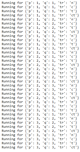
df_results_VARMA.sort_values(by=['RMSE open', 'RMSE high', 'RMSE low', 'RMSE close']).head()
best_values_VARMA = df_results_VARMA.sort_values(by=['RMSE open', 'RMSE high', 'RMSE low', 'RMSE close']).head(1)
best_values_VARMA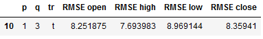
p_value_VARMA = best_values_VARMA['p'].iloc[0]
q_value_VARMA = best_values_VARMA['q'].iloc[0]
tr_value_VARMA = best_values_VARMA['tr'].iloc[0]

print("p_value_VARMA: ", p_value_VARMA)
print("q_value_VARMA: ", q_value_VARMA)
print("tr_value_VARMA: ", tr_value_VARMA)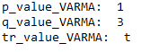
7.2.2 Fit VARMA
model = VARMAX(train_diff,
               order=(p_value_VARMA, q_value_VARMA),trends = tr_value_VARMA).fit(disp=False)
result = model.forecast(steps = len(testX))
7.2.3 Inverse Transformation
df_pred = pd.DataFrame(result, columns=train_diff.columns)
df_pred["new_index"] = range(len(trainX), len(X))
df_pred = df_pred.set_index("new_index")
df_pred.head()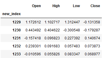
res = inverse_diff_func(trainX, df_pred)
res.head()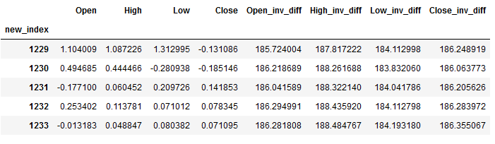
7.2.4 Evaluation of VARMA
for i in ['Open', 'High', 'Low', 'Close']:
    print(f'Evaluation metric for {i}')
    timeseries_evaluation_metrics_func(testX[str(i)] , res[str(i)+'_inv_diff'])
for i in ['Open', 'High', 'Low', 'Close']:

    plt.rcParams["figure.figsize"] = [10,7]
    plt.plot(trainX[str(i)], label='Train '+str(i))
    plt.plot(testX[str(i)], label='Test '+str(i))
    plt.plot(res[str(i)+'_inv_diff'], label='Predicted '+str(i))
    plt.legend(loc='best')
    plt.show()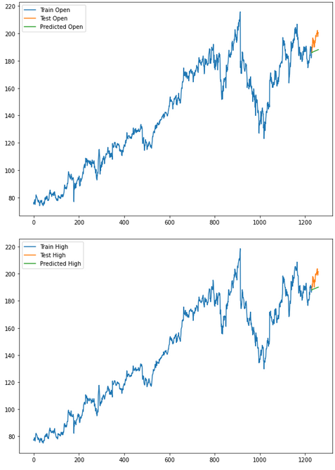
7.3 VARMA with Auto Arima
We can also use the auto_arima function from the pmdarima librarie to determine p and q.
7.3.1 Get best p and q
pq = []
for name, column in train_diff[['Open', 'High', 'Low', 'Close']].iteritems():
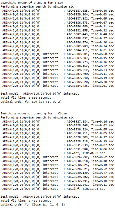
print(f'Searching order of p and q for : {name}')
stepwise_model = auto_arima(train_diff[name],start_p=1, start_q=1,max_p=7, max_q=7, seasonal=False,
trace=True,error_action='ignore',suppress_warnings=True, stepwise=True,maxiter=1000)
parameter = stepwise_model.get_params().get('order')
print(f'optimal order for:{name} is: {parameter} \n\n')
pq.append(stepwise_model.get_params().get('order'))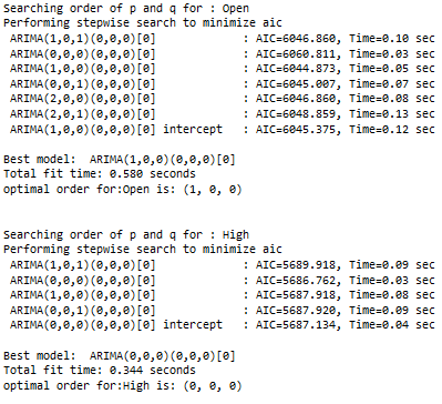
pq
df_results_VARMA_2 = pd.DataFrame(columns=['p', 'q','RMSE Open','RMSE High','RMSE Low','RMSE Close'])

for i in pq:
    if i[0]== 0 and i[2] ==0:
        pass
    else:
        print(f' Running for {i}')
        model = VARMAX(train_diff, order=(i[0],i[2])).fit(disp=False)
        result = model.forecast(steps = len(testX))
        inv_res = inverse_diff_func(trainX, result)
        openrmse = np.sqrt(metrics.mean_squared_error(testX.Open, inv_res.Open_inv_diff))
        highrmse = np.sqrt(metrics.mean_squared_error(testX.High, inv_res.High_inv_diff))
        lowrmse = np.sqrt(metrics.mean_squared_error(testX.Low, inv_res.Low_inv_diff))
        closermse = np.sqrt(metrics.mean_squared_error(testX.Close, inv_res.Close_inv_diff))
        df_results_VARMA_2 = df_results_VARMA_2.append({'p': i[0], 'q': i[2], 'RMSE Open':openrmse,
                                                        'RMSE High':highrmse,'RMSE Low':lowrmse,
                                                        'RMSE Close':closermse }, ignore_index=True)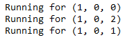
df_results_VARMA_2.sort_values(by=['RMSE Open', 'RMSE High', 'RMSE Low', 'RMSE Close'])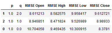
best_values_VAR_2 = df_results_VARMA_2.sort_values(by=['RMSE Open', 'RMSE High',
                                                       'RMSE Low', 'RMSE Close']).head(1)
best_values_VAR_2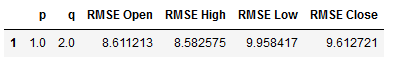
p_value_VARMA_2 = best_values_VAR_2['p'].iloc[0]
q_value_VARMA_2 = best_values_VAR_2['q'].iloc[0]

print("p_value_VARMA_2: ", p_value_VARMA_2)
print("q_value_VARMA_2: ", q_value_VARMA_2)
7.3.2 Fit VARMA_2
model = VARMAX(train_diff,
               order=(int(p_value_VARMA_2),int(q_value_VARMA_2))).fit(disp=False)
result = model.forecast(steps = len(testX))
7.3.3 Inverse Transformation
df_pred = pd.DataFrame(result, columns=train_diff.columns)
df_pred["new_index"] = range(len(trainX), len(X))
df_pred = df_pred.set_index("new_index")
df_pred.head()
res = inverse_diff_func(trainX, df_pred)
res.head()
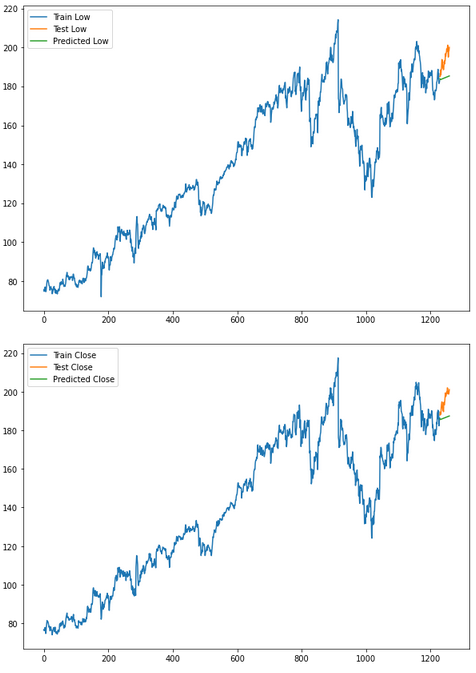
7.3.4 Evaluation of VARMA_2
for i in ['Open', 'High', 'Low', 'Close']:
    print(f'Evaluation metric for {i}')
    timeseries_evaluation_metrics_func(testX[str(i)] , res[str(i)+'_inv_diff'])
for i in ['Open', 'High', 'Low', 'Close' ]:

    plt.rcParams["figure.figsize"] = [10,7]
    plt.plot(trainX[str(i)], label='Train '+str(i))
    plt.plot(testX[str(i)], label='Test '+str(i))
    plt.plot(res[str(i)+'_inv_diff'], label='Predicted '+str(i))
    plt.legend(loc='best')
    plt.show()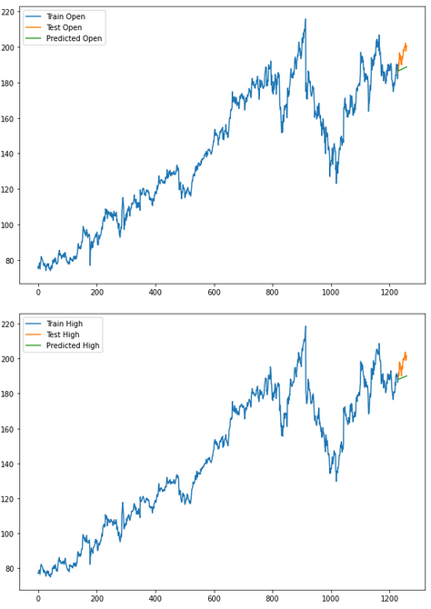
8 Conclusion
Wow another great chapter created! In this post about time series prediction of multiple target variables, I introduced the VAR and VARMA algorithms.
References
The content of this post was inspired by:
Machine Learning Plus: Time Series Analysis in Python – A Comprehensive Guide with Examples from Selva Prabhakaran
Kaggle: Complete Guide on Time Series Analysis in Python from Prashant Banerjee
Vishwas, B. V., & Patel, A. (2020). Hands-on Time Series Analysis with Python. New York: Apress. DOI: 10.1007/978-1-4842-5992-4
Analytics Vidhya: Developing Vector AutoRegressive Model in Python!