1 Introduction

In the past few posts some cluster algorithms were presented. I wrote extensively about “k-Means Clustering”, “Hierarchical Clustering”, “DBSCAN”, “HDBSCAN” and finally about “Gaussian Mixture Models” as well as “Bayesian Gaussian Mixture Models”.

Fortunately, we are not yet through with the most common cluster algorithms. So now we come to affinity propagation.

2 Loading the libraries

import pandas as pd
import numpy as np

# For generating some data
from sklearn.datasets import make_blobs

from matplotlib import pyplot as plt

from sklearn.cluster import AffinityPropagation

from sklearn import metrics

3 Generating some test data

For the following example, I will generate some sample data.

X, y = make_blobs(n_samples=350, centers=4, cluster_std=0.60)
plt.scatter(X[:, 0], X[:, 1], cmap='viridis')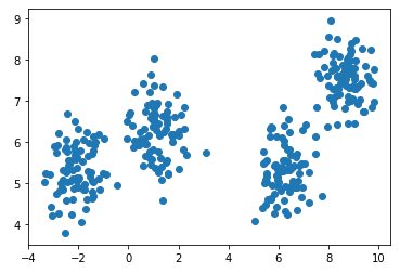

4 Introducing Affinity Propagation

Affinity Propagation was published by Frey and Dueck in 2007, and is only getting more and more popular due to its simplicity, general applicability, and performance. The main drawbacks of k-Means and similar algorithms are having to select the number of clusters (k), and choosing the initial set of points. In contrast to these traditional clustering methods, Affinity Propagation does not require you to specify the number of clusters. Affinity Propagation, instead, takes as input measures of similarity between pairs of data points, and simultaneously considers all data points as potential exemplars.

5 Affinity Propagation with scikit-learn

Now let’s see how Affinity Propagation is used.

afprop  = AffinityPropagation(preference=-50)

afprop.fit(X)

labels = afprop.predict(X)

plt.scatter(X[:, 0], X[:, 1], c=labels, s=40, cmap='viridis')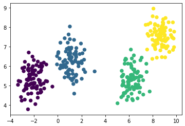

The algorithm worked well.

One the the class attributes is cluster_center_indices_:

cluster_centers_indices = afprop.cluster_centers_indices_
cluster_centers_indices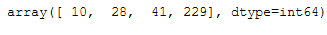

This allows the identified clusters to be calculated.

n_clusters_ = len(cluster_centers_indices)

print('Estimated number of clusters: %d' % n_clusters_)

With the following command we’ll receive the calculated cluster centers:

afprop.cluster_centers_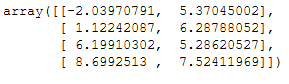

Last but not least some performance metrics:

print('Estimated number of clusters: %d' % n_clusters_)
print("Homogeneity: %0.3f" % metrics.homogeneity_score(y, labels))
print("Completeness: %0.3f" % metrics.completeness_score(y, labels))
print("V-measure: %0.3f" % metrics.v_measure_score(y, labels))
print("Adjusted Rand Index: %0.3f"
      % metrics.adjusted_rand_score(y, labels))
print("Adjusted Mutual Information: %0.3f"
      % metrics.adjusted_mutual_info_score(y, labels))
print("Silhouette Coefficient: %0.3f"
      % metrics.silhouette_score(X, labels, metric='sqeuclidean'))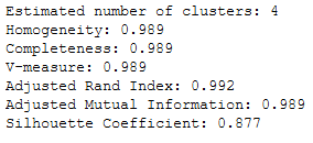

If you want to read the exact description of the metrics see “here”.

6 Conclusion

In this post I explained the affinity propagation algorithm and showed how it can be used with scikit-learn.