1 Introduction
In my last post I reported on “Gaussian Mixture Models”. Now we come to an kind of extension of GMM the Bayesian Gaussian Mixture Models. As we have seen at “GMM”, we could either only infer the number of clusters by eye or by comparing the theoretical information criterions “AIC” and “BIC” for different k.
Rather than manually search for the optimal number of k, you can use the Bayesian Gaussian Mixture Model, which is capable of giving weights equal (or close) to zero to unnecessary cluster. Set the parameter n_components to a value that you have good reason to believe is greater than the optimal number of clusters, and the algorithm will eliminate the unnecessary cluster automatically.
2 Loading the libraries
import pandas as pd
import numpy as np

# For generating some data
from sklearn.datasets import make_blobs

from matplotlib import pyplot as plt

from sklearn.mixture import BayesianGaussianMixture
3 Generating some test data
For the following example, I will generate some sample data.
X, y = make_blobs(n_samples=350, centers=4, cluster_std=0.60)
plt.scatter(X[:, 0], X[:, 1], cmap='viridis')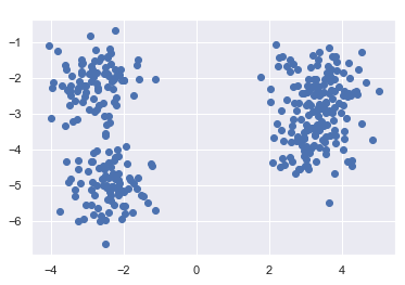
4 Bayesian Gaussian Mixture Models in action
bay_gmm = BayesianGaussianMixture(n_components=10, n_init=10)

bay_gmm.fit(X)
With the following syntax we’ll receive the calculated weights:
bay_gmm_weights = bay_gmm.weights_
np.round(bay_gmm_weights, 2)
As we can see three clusters have been identified. This makes sense after looking at the scatter plot, even though we specified to generate 4 clusters when creating the data. But two clusters are so close together that they were correctly identified as one cluster.
n_clusters_ = (np.round(bay_gmm_weights, 2) > 0).sum()
print('Estimated number of clusters: ' + str(n_clusters_))
Let’s do the predictions:
y_pred = bay_gmm.predict(X)plt.scatter(X[:, 0], X[:, 1], c=y_pred, cmap="viridis")
plt.xlabel("Feature 1")
plt.ylabel("Feature 2")
As with “Gaussian Mixture Models”, we have a ‘predict_proba’ function here.
props = bay_gmm.predict_proba(X)
props = props.round(3)
props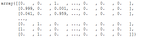
size = 50 * props.max(1) ** 2  # square emphasizes differences
plt.scatter(X[:, 0], X[:, 1], c=y_pred, cmap='viridis', s=size)
In this graphic for the visualization of the probability predictions, we can also see that some points, that have received a lower probability, are shown a little smaller in the graphic.
5 Conclusion
As a supplement to the post “Gaussian Mixture Models”, I have explained in this post how a reasonable number of clusters can be determined with the help of Bayesian Gaussian Mixture Models and how this algorithm can be used.