1 Introduction
After dealing with supervised machine learning models, we now come to another important data science area: unsupervised machine learning models. One class of the unsupervised machine learning models are the cluster algorithms. Clustering algorithms seek to learn, from the properties of the data, an optimal division or discrete labeling of groups of points.
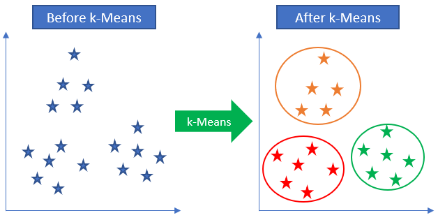
We will start this section with one of the most famous cluster algorithms: k-Means Clustering.
For this post the dataset House Sales in King County, USA from the statistic platform “Kaggle” was used. You can download it from my “GitHub Repository”.
2 Loading the libraries
import pandas as pd
import numpy as np

import matplotlib.pyplot as plt

from sklearn.cluster import KMeans

from sklearn.preprocessing import StandardScaler
from sklearn.preprocessing import MinMaxScaler
3 Introducing k-Means
K-means clustering aims to partition data into k clusters in a way that data points in the same cluster are similar and data points in the different clusters are farther apart. In other words, the K-means algorithm identifies k number of centroids, and then allocates every data point to the nearest cluster, while keeping the centroids as small as possible.
There are many methods to measure the distance. Euclidean distance is one of most commonly used distance measurements.
How the K-means algorithm works
To process the learning data, the K-means algorithm in data mining starts with a first group of randomly selected centroids, which are used as the beginning points for every cluster, and then performs iterative calculations to optimize the positions of the centroids.
4 Preparation of the data record
At the beginning we throw unnecessary variables out of the data set.
house = pd.read_csv("path/to/file/houce_prices.csv")
house = house.drop(['id', 'date', 'zipcode', 'lat', 'long'], axis=1)
house.head()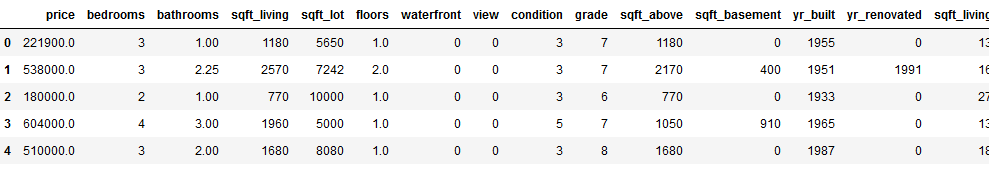
Now we are creating a new target variable. To do this we look at a histogram that shows house prices.
plt.hist(house['price'], bins='auto')
plt.title("Histogram for house prices")
plt.xlim(xmin=0, xmax = 1200000)
plt.show()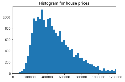
Now we have a rough idea of how we could divide house prices into three categories: cheap, medium and expensive. To do so we’ll use the following function:
def house_price_cat(df):

    if (df['price'] >= 600000):
        return 'expensive'

    elif (df['price'] < 600000) and (df['price'] > 300000):
        return 'medium'

    elif (df['price'] <= 300000):
        return 'cheap'
house['house_price_cat'] = house.apply(house_price_cat, axis = 1)
house.head()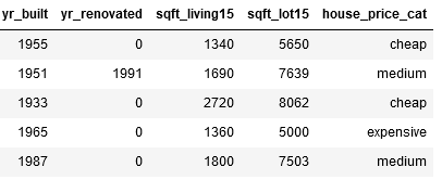
As we can see, we now have a new column with three categories of house prices.
house['house_price_cat'].value_counts().T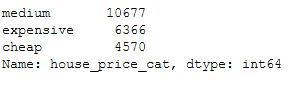
For our further procedure we convert these into numerical values. There are several ways to do so. If you are interested in the different methods, check out this post from me: “Types of Encoder”
ord_house_price_dict = {'cheap' : 0,
                        'medium' : 1,
                        'expensive' : 2}

house['house_price_Ordinal'] = house.house_price_cat.map(ord_house_price_dict)
house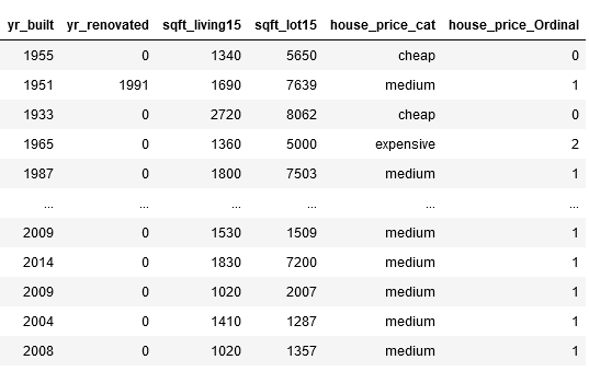
Now let’s check for missing values:
def missing_values_table(df):
        # Total missing values
        mis_val = df.isnull().sum()

        # Percentage of missing values
        mis_val_percent = 100 * df.isnull().sum() / len(df)

        # Make a table with the results
        mis_val_table = pd.concat([mis_val, mis_val_percent], axis=1)

        # Rename the columns
        mis_val_table_ren_columns = mis_val_table.rename(
        columns = {0 : 'Missing Values', 1 : '% of Total Values'})

        # Sort the table by percentage of missing descending
        mis_val_table_ren_columns = mis_val_table_ren_columns[
            mis_val_table_ren_columns.iloc[:,1] != 0].sort_values(
        '% of Total Values', ascending=False).round(1)

        # Print some summary information
        print ("Your selected dataframe has " + str(df.shape[1]) + " columns.\n"
            "There are " + str(mis_val_table_ren_columns.shape[0]) +
              " columns that have missing values.")

        # Return the dataframe with missing information
        return mis_val_table_ren_columns

missing_values_table(house)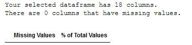
No one, perfect.
Last but not least the train test split:
x = house.drop(['house_price_cat', 'house_price_Ordinal'], axis=1)
y = house['house_price_Ordinal']
trainX, testX, trainY, testY = train_test_split(x, y, test_size = 0.2)
And the conversion to numpy arrays:
trainX = np.array(trainX)
trainY = np.array(trainY)
5 Application of k-Means
Since we know that we are looking for 3 clusters (cheap, medium and expensive), we set k to 3.
kmeans = KMeans(n_clusters=3)
kmeans.fit(trainX)
correct = 0
for i in range(len(trainX)):
    predict_me = np.array(trainX[i].astype(float))
    predict_me = predict_me.reshape(-1, len(predict_me))
    prediction = kmeans.predict(predict_me)
    if prediction[0] == trainY[i]:
        correct += 1

print(correct/len(trainX))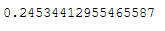
24.5 % accuracy … Not really a very good result but sufficient for illustrative purposes.
Let’s try to increase the max. iteration parameter.
kmeans = KMeans(n_clusters=3, max_iter=600, algorithm = 'auto')
kmeans.fit(trainX)
correct = 0
for i in range(len(trainX)):
    predict_me = np.array(trainX[i].astype(float))
    predict_me = predict_me.reshape(-1, len(predict_me))
    prediction = kmeans.predict(predict_me)
    if prediction[0] == trainY[i]:
        correct += 1

print(correct/len(trainX))
No improvement. What a shame.
Maybe it’s because we didn’t scale the data. Let’s try this next. If you are interested in the various scaling methods available, check out this post from me: “Feature Scaling with Scikit-Learn”
sc=StandardScaler()

trainX_scaled = sc.fit_transform(trainX)
kmeans = KMeans(n_clusters=3)
kmeans.fit(trainX_scaled)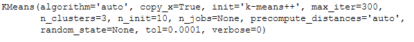
correct = 0
for i in range(len(trainX_scaled)):
    predict_me = np.array(trainX_scaled[i].astype(float))
    predict_me = predict_me.reshape(-1, len(predict_me))
    prediction = kmeans.predict(predict_me)
    if prediction[0] == trainY[i]:
        correct += 1

print(correct/len(trainX_scaled))
This worked. Improvement of 13%.
6 Determine the optimal k for k-Means
This time we knew how many clusters to look for. But k-Means is actually an unsupervised machine learning algorithm. But also here are opportunities to see which k best fits our data. One of them is the ‘Elbow-Method’.
To do so we have to remove the specially created target variables from the current record.
house = house.drop(['house_price_cat', 'house_price_Ordinal'], axis=1)
house.head()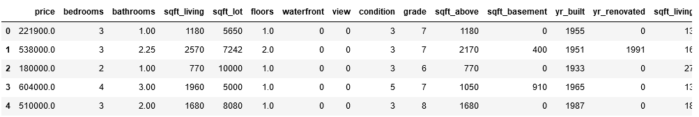
We also scale the data again (this time with the MinMaxScaler).
mms = MinMaxScaler()
mms.fit(house)
data_transformed = mms.transform(house)
Sum_of_squared_distances = []
K = range(1,15)
for k in K:
km = KMeans(n_clusters=k)
km = km.fit(data_transformed)
Sum_of_squared_distances.append(km.inertia_)plt.plot(K, Sum_of_squared_distances, 'bx-')
plt.xlabel('k')
plt.ylabel('Sum_of_squared_distances')
plt.title('Elbow Method For Optimal k')
plt.show()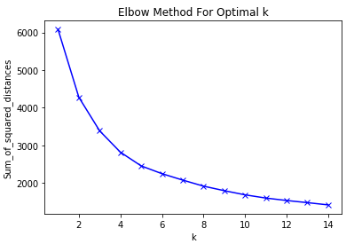
As we can see the optimal k for this dataset is 5. Let’s use this k for our final k-Mean algorithm.
km = KMeans(n_clusters=5, random_state=1)
km.fit(house)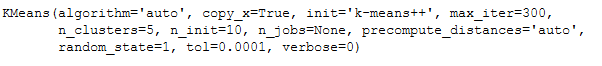
We can now assign the calculated clusters to the observations from the original data set.
predict=km.predict(house)
house['my_clusters'] = pd.Series(predict, index=house.index)
house.head()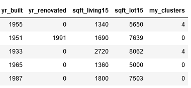
Here is an overview of the respective size of the clusters created.
house['my_clusters'].value_counts()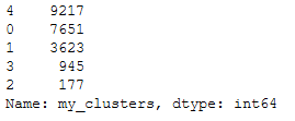
7 Visualization
df_sub = house[['sqft_living', 'price']].valuesplt.scatter(df_sub[predict==0, 0], df_sub[predict==0, 1], s=100, c='red', label ='Cluster 1')
plt.scatter(df_sub[predict==1, 0], df_sub[predict==1, 1], s=100, c='blue', label ='Cluster 2')
plt.scatter(df_sub[predict==2, 0], df_sub[predict==2, 1], s=100, c='green', label ='Cluster 3')
plt.scatter(df_sub[predict==3, 0], df_sub[predict==3, 1], s=100, c='cyan', label ='Cluster 4')
plt.scatter(df_sub[predict==4, 0], df_sub[predict==4, 1], s=100, c='magenta', label ='Cluster 5')
#plt.scatter(km.cluster_centers_[:, 0], km.cluster_centers_[:, 1], s=300, c='yellow', label = 'Centroids')
#plt.scatter()
plt.title('Cluster of Houses')
plt.xlim((0, 8000))
plt.ylim((0,4000000))
plt.xlabel('sqft_living \n\n Cluster1(Red), Cluster2 (Blue), Cluster3(Green), Cluster4(Cyan), Cluster5 (Magenta)')
plt.ylabel('Price')
plt.show()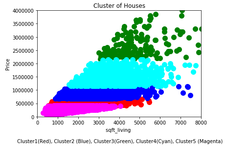
8 Conclusion
As with any machine learning algorithm, there are advantages and disadvantages:
Advantages of k-Means
- Relatively simple to implement
- Scales to large data sets
- Easily adapts to new examples
- Generalizes to clusters of different shapes and sizes, such as elliptical clusters
Disadvantages of k-Means
- Choosing manually
- Being dependent on initial values
- Clustering data of varying sizes and density
- Clustering outliers