1 Introduction

The next unsupervised machine learning cluster algorithms is the Density-Based Spatial Clustering and Application with Noise (DBSCAN). DBSCAN is a density-based clusering algorithm, which can be used to identify clusters of any shape in a data set containing noise and outliers.

2 Loading the libraries

import pandas as pd
import numpy as np
import matplotlib.pyplot as plt
from sklearn.datasets import make_blobs

from sklearn.preprocessing import StandardScaler

from sklearn.cluster import KMeans
from sklearn.cluster import DBSCAN

from sklearn.metrics.cluster import adjusted_rand_score

3 Introducing DBSCAN

The basic idea behind DBSCAN is derived from a human intuitive clustering method.

If you have a look at the picture below you can easily identify 2 clusters along with several points of noise, because of the differences in the density of points.

Clusters are dense regions in the data space, separated by regions of lower density of points. The Density-Based Spatial Clustering and Application with Noise algorithm is based on this intuitive notion of “clusters” and “noise”. The key idea is that for each point of a cluster, the neighborhood of a given radius has to contain at least a minimum number of points.

4 DBSCAN with Scikit-Learn

In the following I will show you an example of some of the strengths of DBSCAN clustering when k-means clustering doesn’t seem to handle the data shape well.

4.1 Data preparation

For an illustrative example, I will create a data set artificially.

# generate some random cluster data
X, y = make_blobs(random_state=170, n_samples=500, centers = 5)

# transform the data to be stretched
rng = np.random.RandomState(74)
transformation = rng.normal(size=(2, 2))
X = np.dot(X, transformation)

plt.scatter(X[:, 0], X[:, 1])
plt.xlabel("Feature 1")
plt.ylabel("Feature 2")
plt.show()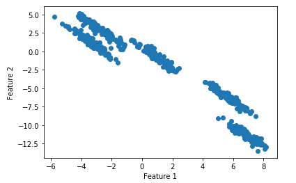

# scaling the data
scaler = StandardScaler()
X_scaled = scaler.fit_transform(X)

4.2 k-Means

If you want to find out exactly how k-Means works have a look at this post of mine: “k-Means Clustering”

# cluster the data into five clusters
kmeans = KMeans(n_clusters=5)
kmeans.fit(X_scaled)
y_pred = kmeans.predict(X_scaled)

# plot the cluster assignments and cluster centers

plt.scatter(X[:, 0], X[:, 1], c=y_pred, cmap="viridis")
plt.xlabel("Feature 1")
plt.ylabel("Feature 2")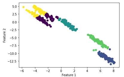

We can measure the performance with the adjusted_rand_score

#k-means performance:
print("ARI =", adjusted_rand_score(y, y_pred))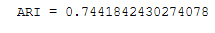

4.3 DBSCAN

# cluster the data into five clusters
dbscan = DBSCAN(eps=0.123, min_samples = 2)

clusters = dbscan.fit_predict(X_scaled)

# plot the cluster assignments
plt.scatter(X[:, 0], X[:, 1], c=clusters, cmap="viridis")
plt.xlabel("Feature 1")
plt.ylabel("Feature 2")

#DBSCAN performance:
print("ARI =", adjusted_rand_score(y, clusters))

Here we see that the performance of the DBSCANS is much higher than k-means with this data set.

Let’s have a look at the labels:

labels = dbscan.labels_
labels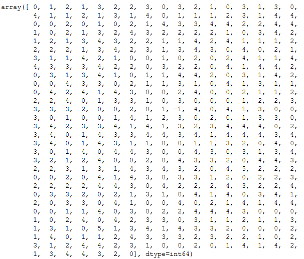

We can also add them to the original record.

X_df = pd.DataFrame(X)
db_cluster = pd.DataFrame(labels)  

df = pd.concat([X_df, db_cluster], axis=1)
df.columns = ['Feature 1', 'Feature 2', 'db_cluster']
df.head()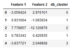

Let’s have a detailed look at the generated clusters:

view_cluster = df['db_cluster'].value_counts().T
view_cluster = pd.DataFrame(data=view_cluster)
view_cluster = view_cluster.reset_index()
view_cluster.columns = ['db_cluster', 'count']
view_cluster.sort_values(by='db_cluster', ascending=False)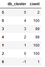

As we can see from the overview above, a point was assigned to cluster -1. This is not a cluster at all, it’s a noisy point.

# Number of clusters in labels, ignoring noise if present.
n_clusters_ = len(set(labels)) - (1 if -1 in labels else 0)
print('Estimated number of clusters: %d' % n_clusters_)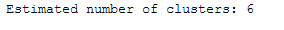

5 Conclusion

The example in this post showed that clustering also depends heavily on the distribution of the data points and that it is always worth trying out several cluster algorithms.