1 Introduction
In the series of unsupervised learning cluster algorithms, we have already got to know “hierarchical clustering” and “density-based clustering (DBSCAN)”. Now we come to an expansion of the DBSCAN algorithm in which the hierarchical approach is integrated. So called: Hierarchical Density-Based Spatial Clustering and Application with Noise (HDBSCAN)
2 Loading the libraries
import numpy as np
import pandas as pd

from sklearn.datasets import load_digits


from sklearn.manifold import TSNE
import hdbscan

from sklearn.datasets import make_blobs
from sklearn.datasets import make_moons

import matplotlib.pyplot as plt
import seaborn as sns
plot_kwds = {'alpha' : 0.25, 's' : 10, 'linewidths':0}
3 Introducing HDBSCAN
We already know from “DBSCAN” post this algorithm needs a minimum cluster size and a distance threshold epsilon as user-defined input parameters. HDBSCAN is basically a DBSCAN implementation for varying epsilon values and therefore only needs the minimum cluster size as single input parameter. Unlike DBSCAN, this allows to it find clusters of variable densities without having to choose a suitable distance threshold first.
HDBSCAN extends DBSCAN by converting it into a hierarchical clustering algorithm, and then using a technique to extract a flat clustering based in the stability of clusters.
4 Parameter Selection for HDBSCAN
While the HDBSCAN class has a large number of parameters that can be set on initialization, in practice there are a very small number of parameters that have significant practical effect on clustering.
One of these is the min_cluster_size.
The “digits” dataset from scikit learn is used to illustrate the effects of the following changes to the parameters.
digits = load_digits()
data = digits.data
The loaded data set contains 64 dimensions. For a visual representation, I use t-SNE (t-distributed Stochastic Neighbor Embedding) in advance. I will explain the exact functioning of this algorithm for dimension reduction in a separate post.
projection = TSNE().fit_transform(data)
plt.scatter(*projection.T, **plot_kwds)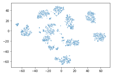
This is what a two-dimensional representation of our digits dataset looks like.
The min_cluster_size parameter is a relatively intuitive parameter to select. Set it to the smallest size grouping that you wish to consider a cluster.
In the following we will see how the calculated number of clusters will change from varying the min_cluster_size. I will start with a min_cluster_size of 15.
clusterer = hdbscan.HDBSCAN(min_cluster_size=15).fit(data)color_palette = sns.color_palette('Paired', 12)
cluster_colors = [color_palette[x] if x >= 0
else (0.5, 0.5, 0.5)
for x in clusterer.labels_]
cluster_member_colors = [sns.desaturate(x, p) for x, p in
zip(cluster_colors, clusterer.probabilities_)]
plt.scatter(*projection.T, s=20, linewidth=0, c=cluster_member_colors, alpha=0.25)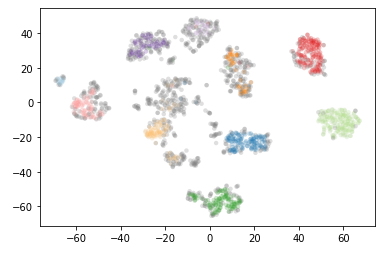
labels = clusterer.labels_# Number of clusters in labels, ignoring noise if present.
n_clusters_ = len(set(labels)) - (1 if -1 in labels else 0)
print('Estimated number of clusters: %d' % n_clusters_)
10 estimated clusters. Now let’s see what happens if we increase the min_cluster_size to 30.
clusterer = hdbscan.HDBSCAN(min_cluster_size=30).fit(data)
color_palette = sns.color_palette('Paired', 12)
cluster_colors = [color_palette[x] if x >= 0
                  else (0.5, 0.5, 0.5)
                  for x in clusterer.labels_]
cluster_member_colors = [sns.desaturate(x, p) for x, p in
                         zip(cluster_colors, clusterer.probabilities_)]
plt.scatter(*projection.T, s=20, linewidth=0, c=cluster_member_colors, alpha=0.25)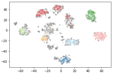
labels = clusterer.labels_
# Number of clusters in labels, ignoring noise if present.
n_clusters_ = len(set(labels)) - (1 if -1 in labels else 0)
print('Estimated number of clusters: %d' % n_clusters_)
We see if we increase the parameter min_cluster_size the number of clusters found decreases. Let’s see what happens at min_cluster_size 60.
clusterer = hdbscan.HDBSCAN(min_cluster_size=60).fit(data)
color_palette = sns.color_palette('Paired', 12)
cluster_colors = [color_palette[x] if x >= 0
else (0.5, 0.5, 0.5)
for x in clusterer.labels_]
cluster_member_colors = [sns.desaturate(x, p) for x, p in
zip(cluster_colors, clusterer.probabilities_)]
plt.scatter(*projection.T, s=20, linewidth=0, c=cluster_member_colors, alpha=0.25)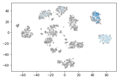
labels = clusterer.labels_

# Number of clusters in labels, ignoring noise if present.
n_clusters_ = len(set(labels)) - (1 if -1 in labels else 0)
print('Estimated number of clusters: %d' % n_clusters_)
Only two clusters are still being calculated. These two clusters are known as really core clusters. But actually, more than two clusters should contain more than 60 assigned data points. So why is so much data spotted as noisy data points? The answer is that HDBSCAN has a second parameter min_samples. The implementation defaults this value (if it is unspecified) to whatever min_cluster_size is set to. We can recover some of our original clusters by explicitly providing min_samples at the original value of 15.
clusterer = hdbscan.HDBSCAN(min_cluster_size=60, min_samples=15).fit(data)
color_palette = sns.color_palette('Paired', 12)
cluster_colors = [color_palette[x] if x >= 0
else (0.5, 0.5, 0.5)
for x in clusterer.labels_]
cluster_member_colors = [sns.desaturate(x, p) for x, p in
zip(cluster_colors, clusterer.probabilities_)]
plt.scatter(*projection.T, s=20, linewidth=0, c=cluster_member_colors, alpha=0.25)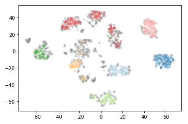
labels = clusterer.labels_

# Number of clusters in labels, ignoring noise if present.
n_clusters_ = len(set(labels)) - (1 if -1 in labels else 0)
print('Estimated number of clusters: %d' % n_clusters_)
As you can see this results in us recovering something much closer to our original clustering, only now with some of the smaller clusters pruned out.
Since we have seen that min_samples clearly has a dramatic effect on clustering, the question becomes: how do we select this parameter? The simplest intuition for what min_samples does is provide a measure of how conservative you want you clustering to be. The larger the value of min_samples you provide, the more conservative the clustering – more points will be declared as noise, and clusters will be restricted to progressively more dense areas. We can see this in practice by leaving the min_cluster_size at 60, but reducing min_samples to 1.
clusterer = hdbscan.HDBSCAN(min_cluster_size=60, min_samples=1).fit(data)
color_palette = sns.color_palette('Paired', 12)
cluster_colors = [color_palette[x] if x >= 0
else (0.5, 0.5, 0.5)
for x in clusterer.labels_]
cluster_member_colors = [sns.desaturate(x, p) for x, p in
zip(cluster_colors, clusterer.probabilities_)]
plt.scatter(*projection.T, s=20, linewidth=0, c=cluster_member_colors, alpha=0.25)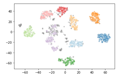
labels = clusterer.labels_

# Number of clusters in labels, ignoring noise if present.
n_clusters_ = len(set(labels)) - (1 if -1 in labels else 0)
print('Estimated number of clusters: %d' % n_clusters_)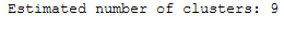
5 HDBSCAN in action
To see how HDBSCAN works we’ll generate some data again.
Xmoon, ymoon = make_moons(80, noise=.06)
X, y = make_blobs(n_samples=50, centers=[(-0.75,2.25), (1.0, 2.0)], n_features=2, cluster_std=0.25)

test_data = np.vstack([Xmoon, X])

plt.scatter(test_data.T[0], test_data.T[1], color='b', **plot_kwds)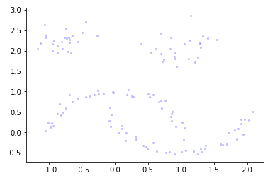
5.1 Functionality of the HDBSCAN algorithm
The functionality of the HDBSCAN algorithm can be described in the following steps:
- Transform the space according to the density/sparsity
- Build the minimum spanning tree of the distance weighted graph
- Construct a cluster hierarchy of connected components
- Condense the cluster hierarchy based on minimum cluster size
- Extract the stable clusters from the condensed tree
Ok let’s train and fit our model:
clusterer = hdbscan.HDBSCAN(min_cluster_size=5, gen_min_span_tree=True)
clusterer.fit(test_data)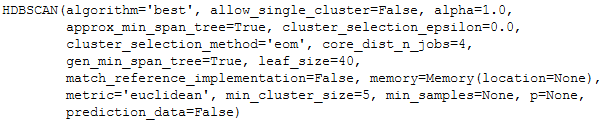
5.2 Visualization options
For most of the above named steps, the hdbscan library offers its own visualization options. If you want to do this, don’t forget to set the gen_min_span_tree parameter to True.
Build the minimum spanning tree
clusterer.minimum_spanning_tree_.plot(edge_cmap='viridis',
                                      edge_alpha=0.6,
                                      node_size=80,
                                      edge_linewidth=2)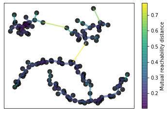
Build the cluster hierarchy
clusterer.single_linkage_tree_.plot(cmap='viridis', colorbar=True)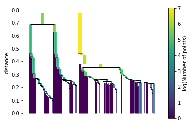
Condense the cluster tree
clusterer.condensed_tree_.plot()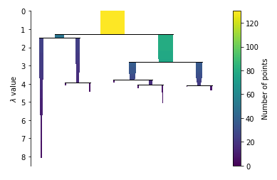
Extract the clusters
clusterer.condensed_tree_.plot(select_clusters=True, selection_palette=sns.color_palette())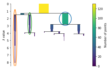
Visualize the colculated clusters
palette = sns.color_palette()
cluster_colors = [sns.desaturate(palette[col], sat)
                  if col >= 0 else (0.5, 0.5, 0.5) for col, sat in
                  zip(clusterer.labels_, clusterer.probabilities_)]
plt.scatter(test_data.T[0], test_data.T[1], c=cluster_colors, **plot_kwds)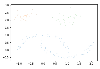
I personally find this representation not so clear from the visual point of view. We can do better. So let’s bring out test_data and the calculated hdb_cluster together:
df = pd.DataFrame(test_data)
df.columns = ['Value_1', 'Value_2']
df.head()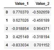
labels = clusterer.labels_hdb_cluster = pd.DataFrame(labels)
df = pd.concat([df, hdb_cluster], axis=1)
df.columns = ['Value_1', 'Value_2', 'hdb_cluster']
df.head()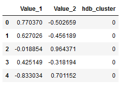
plt.scatter(df['Value_1'], df['Value_2'], c=labels, s=40, cmap='viridis')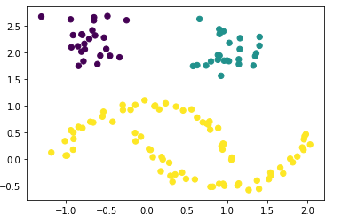
Now it is clearly shown.
5.3 Predictions with HDBSCAN
Similar to the visualization of the individual steps regarding the functioning of HDBSCAN, the prediction_data parameter must be set to True so that we can use the model to make predictions for new data. In the following I set this parameter accodingly and also fit the model on our test_data.
clusterer = hdbscan.HDBSCAN(min_cluster_size=5, prediction_data=True).fit(test_data)After this step I create some new data points:
df_new = pd.DataFrame({'Col1': [0, 1.5],
                   'Col2': [1.5, 1]})
df_new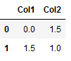
If you have a single point be sure to wrap it in a list.
test_points = np.array(df_new)
test_points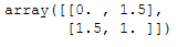
With the approximate_predict function we’ll get the labels for our new data.
test_labels, strengths = hdbscan.approximate_predict(clusterer, test_points)
test_labels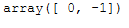
We also add these predictions to the dataframe (df_new).
hdb2_cluster = pd.DataFrame(test_labels)
df_new = pd.concat([df_new, hdb2_cluster], axis=1)
df_new.columns = ['Value_1', 'Value_2', 'hdb_cluster']
df_new.head()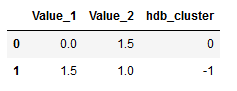
Now let’s connect the original dataframe with the new dataframe:
data_frames = [df, df_new]

df_final = pd.concat(data_frames)
df_final.tail()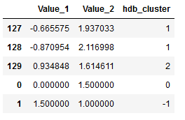
In the above overview I showed the last 5 rows of the final dataframe. As we can see, the two additional points were listed along with their assigned cluster. Let’s take a look at how many clusters have been identified.
df_final['hdb_cluster'].value_counts()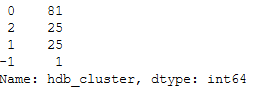
3 clusters were identified. Remember that a point was labeled -1. This is not a separate cluster but a noisy point.
Now we age going to visualize the final dataframe and pay attention to the two new points.
plt.scatter(df_final['Value_1'], df_final['Value_2'], c=df_final['hdb_cluster'], s=40, cmap='viridis')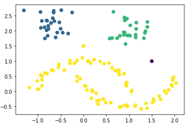
You can see very nicely that the first point (0, 1.5) was assigned to the yellow cluster and the second point (1.5, 1) is shown as an outlier. In the diagram below, I have shown the exact location using red and green lines.
plt.scatter(df_final['Value_1'], df_final['Value_2'], c=df_final['hdb_cluster'], s=40, cmap='viridis')

plt.axhline(y=1, color='r', linestyle='--')
plt.axvline(x=1.5, color='r', linestyle='--')

plt.axhline(y=1.5, color='g', linestyle='--')
plt.axvline(x=0, color='g', linestyle='--')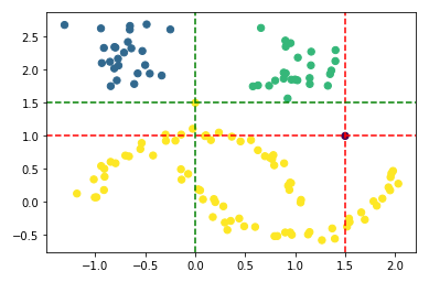
6 Conclustion
Like the DBSCAN algorithm, the HDBSCAN algorithm is a density-based unsupervised machine learning algorithm and can be viewed as an extension of this. It may seem somewhat complicated – there are a fair number of moving parts to the algorithm – but ultimately each part is actually very straightforward and can be optimized well.