1 Introduction

Let’s come to a further unsupervised learning cluster algorithm: The Gaussian Mixture Models. As simple or good as the K-Means algorithm is, it is often difficult to use in real world situations. In particular, the non-probabilistic nature of k-means and its use of simple distance-from-cluster-center to assign cluster membership leads to poor performance for many real-world problems. Therefore I will give you an overview of Gaussian mixture models (GMMs), which can be viewed as an extension of the ideas behind k-means, but can also be a powerful tool for estimation beyond simple clustering.

2 Loading the libraries

import pandas as pd
import numpy as np

import matplotlib.pyplot as plt
%matplotlib inline
import seaborn as sns; sns.set()

# For generating some data
from sklearn.datasets import make_blobs


from sklearn.cluster import KMeans
from sklearn import mixture

# For creating some circles around the center of each cluster within the visualizations
from scipy.spatial.distance import cdist
# For creating some circles for probability area around the center of each cluster within the visualizations
from matplotlib.patches import Ellipse

3 Generating some test data

For the following example, in which I will show which weaknesses there are in k-means, I will generate some sample data.

X, y = make_blobs(n_samples=350, centers=4, n_features=2, cluster_std=0.67)
X = X[:, ::-1] # flip axes for better plotting
plt.scatter(X[:, 0], X[:, 1], cmap='viridis')

4 Weaknesses of k-Means

In the graphic above we can see with the eye that there are probably 3-4 clusters. So let’s calculate k-Means with 4 clusters.

kmeans = KMeans(n_clusters=4)
kmeans.fit(X)
labels = kmeans.predict(X)

plt.scatter(X[:, 0], X[:, 1], c=labels, s=40, cmap='viridis')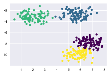

At this point, k-means determined the clusters quite well. Once you understand how k-means works, you know that this algorithm only includes the points within its calculated radius in a cluster. We can visualize these radii.

#Keep in mind to change n_clusters accordingly

def plot_kmeans(kmeans, X, n_clusters=4, rseed=0, ax=None):
    labels = kmeans.fit_predict(X)

    # plot the input data
    ax = ax or plt.gca()
    ax.axis('equal')
    ax.scatter(X[:, 0], X[:, 1], c=labels, s=40, cmap='viridis', zorder=2)

    # plot the representation of the KMeans model
    centers = kmeans.cluster_centers_
    radii = [cdist(X[labels == i], [center]).max()
             for i, center in enumerate(centers)]
    for c, r in zip(centers, radii):
        ax.add_patch(plt.Circle(c, r, fc='#CCCCCC', lw=3, alpha=0.5, zorder=1))

kmeans = KMeans(n_clusters=4)
plot_kmeans(kmeans, X)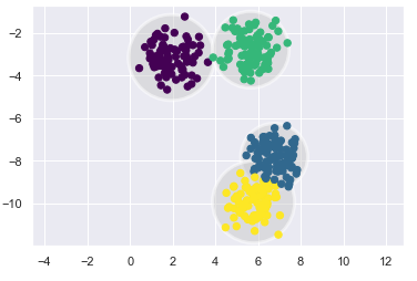

An important observation for k-Means is that these cluster models must be circular. k-Means has no built-in way of accounting for oblong or elliptical clusters. So, let’s see how k-Means work with less orderly data.

# transform the data to be stretched
rng = np.random.RandomState(74)
transformation = rng.normal(size=(2, 2))
X_stretched = np.dot(X, transformation)

kmeans = KMeans(n_clusters=4)
plot_kmeans(kmeans, X_stretched)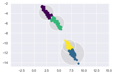

You can see that this can quickly lead to problems.

5 Gaussian Mixture Models

A Gaussian mixture model (GMM) attempts to find a mixture of multi-dimensional Gaussian probability distributions that best model any input dataset. In the simplest case, GMMs can be used for finding clusters in the same manner as k-Means. Now let’s see how the GMM model works.

gmm = mixture.GaussianMixture(n_components=4)
gmm.fit(X)
labels = gmm.predict(X)

plt.scatter(X[:, 0], X[:, 1], c=labels, s=40, cmap='viridis')

But because gaussian mixture model contains a probabilistic model under the hood, it is also possible to find probabilistic cluster assignments. In Scikit-Learn this is done using the predict_proba method.

probs = gmm.predict_proba(X)
probs

For a better view we’ll round it:

props = probs.round(3)
props

We can also visualize the effect of the probabilities.

size = 50 * probs.max(1) ** 2  # square emphasizes differences
plt.scatter(X[:, 0], X[:, 1], c=labels, cmap='viridis', s=size)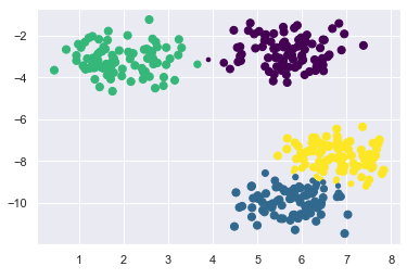

As you can see now, points that are more likely to belong to the respective cluster are shown smaller than the others. Here we can visually represent the probability areas in which the more distant points lie, too.

def draw_ellipse(position, covariance, ax=None, **kwargs):
    """Draw an ellipse with a given position and covariance"""
    ax = ax or plt.gca()
    
    # Convert covariance to principal axes
    if covariance.shape == (2, 2):
        U, s, Vt = np.linalg.svd(covariance)
        angle = np.degrees(np.arctan2(U[1, 0], U[0, 0]))
        width, height = 2 * np.sqrt(s)
    else:
        angle = 0
        width, height = 2 * np.sqrt(covariance)
    
    # Draw the Ellipse
    for nsig in range(1, 4):
        ax.add_patch(Ellipse(position, nsig * width, nsig * height, angle, **kwargs))
        
def plot_gmm(gmm, X, label=True, ax=None):
    ax = ax or plt.gca()
    labels = gmm.fit(X).predict(X)
    if label:
        ax.scatter(X[:, 0], X[:, 1], c=labels, s=40, cmap='viridis', zorder=2)
    else:
        ax.scatter(X[:, 0], X[:, 1], s=40, zorder=2)
    ax.axis('equal')
    
    w_factor = 0.2 / gmm.weights_.max()
    for pos, covar, w in zip(gmm.means_, gmm.covariances_, gmm.weights_):
        draw_ellipse(pos, covar, alpha=w * w_factor)

gmm = mixture.GaussianMixture(n_components=4)
plot_gmm(gmm, X)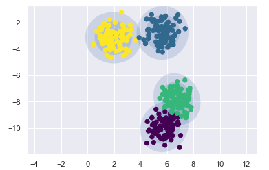

Similarly, we can use the GMM approach to fit our stretched dataset. Allowing for a full covariance the model will fit even very oblong, stretched-out clusters:

gmm = mixture.GaussianMixture(n_components=4, covariance_type='full')
plot_gmm(gmm, X_stretched)

6 Determine the optimal k for GMM

With k-Means, you could use the inertia or silhouette score to select the appropriate number of clusters. But with GMM, it’s not possible to use these metrics because they are not reliable when clusters are not spherical or have different sizes. Instead you can try to find the model that minimizes a theoretical information criterion, such as “AIC” or “BIC”.

Let’s create for this some new sample data:

X, y = make_blobs(n_samples=350, centers=3, cluster_std=0.67)
X = X[:, ::-1] # flip axes for better plotting
plt.scatter(X[:, 0], X[:, 1], cmap='viridis')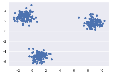

We have three clusters that are easy to recognize. therefore, we can determine k fairly safely by eye.

gmm = mixture.GaussianMixture(n_components=3)
gmm.fit(X)
labels = gmm.predict(X)

plt.scatter(X[:, 0], X[:, 1], c=labels, s=40, cmap='viridis')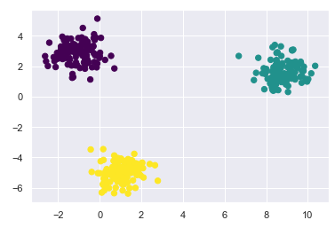

Now we try to find out with BIC and AIC whether this calculation and comparison would have come to the same result.

Sum_bic = []
Sum_aic = []

K = range(1,8)
for k in K:
    gmm = mixture.GaussianMixture(n_components=k)
    gmm = gmm.fit(X)
    Sum_bic.append(gmm.bic(X))
    Sum_aic.append(gmm.aic(X))

x1 = K
y1 = Sum_aic
plt.plot(x1, y1, label = "AIC")
x2 = K
y2 = Sum_bic
plt.plot(x2, y2, label = "BIC")

plt.title("AIC and BIC for dofferent numbers of k", fontsize=16, fontweight='bold')
plt.xlabel("k")
plt.ylabel("Information Criterion")
plt.legend(loc='upper right')
plt.show()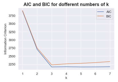

BIC and AIC also have their minimum at k = 3.

7 GMM for density estimation

GMM is often used / viewed as a cluster algorithm. Fundamentally it is an algorithm for density estimation. That is to say, the result of a GMM fit to some data is technically not a clustering model, but a generative probabilistic model describing the distribution of the data.

Let me give you an example with Scikit-Learn’s make_moons function:

from sklearn.datasets import make_moons

Xmoon, ymoon = make_moons(300, noise=.06)
plt.scatter(Xmoon[:, 0], Xmoon[:, 1])

If I try to fit this with a two-component GMM viewed as a clustering model, the results are not particularly useful.

gmm = mixture.GaussianMixture(n_components=2, covariance_type='full')
plot_gmm(gmm, Xmoon)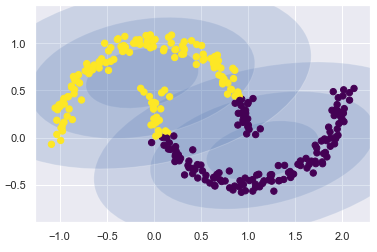

But if I instead use many more components and ignore the cluster labels, we find a fit that is much closer to the input data.

gmm = mixture.GaussianMixture(n_components=18, covariance_type='full')
plot_gmm(gmm, Xmoon, label=False)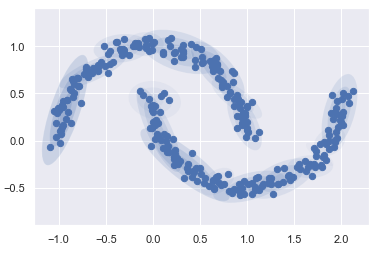

No clustering should take place here, but rather the overall distribution of the available data should be found. We can use a fitted GMM model to generate new random data distributed similarly to our input.

gmm = mixture.GaussianMixture(n_components=18)
gmm.fit(Xmoon)


[Xnew, Ynew] = gmm.sample(400)
plt.scatter(Xnew[:, 0], Xnew[:, 1])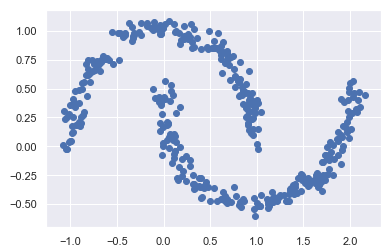

Here we can see 400 new generated data poinst. It looks very similar to the orginal data frame, doesn’t it?

We can also determine the number of components we need:

n_components = np.arange(1, 25)
models = [mixture.GaussianMixture(n, covariance_type='full').fit(Xmoon)
          for n in n_components]

plt.plot(n_components, [m.bic(Xmoon) for m in models], label='BIC')
plt.plot(n_components, [m.aic(Xmoon) for m in models], label='AIC')
plt.legend(loc='best')
plt.xlabel('n_components')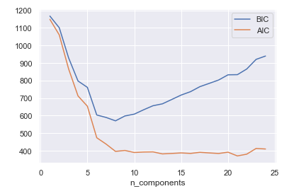

Based on the graphic, I choose 9 components to use.

gmm = mixture.GaussianMixture(n_components=9, covariance_type='full')
plot_gmm(gmm, Xmoon, label=False)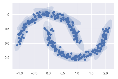

gmm = mixture.GaussianMixture(n_components=9)
gmm.fit(Xmoon)


[Xnew, Ynew] = gmm.sample(400)

plt.scatter(Xnew[:, 0], Xnew[:, 1])

Notice: this choice of number of components measures how well GMM works as a density estimator, not how well it works as a clustering algorithm.

8 Conclusion

In this post I showed the weaknesses of the K-Means algorithm and illustrated how GMMs can still be used to identify more difficult patterns in data.