1 Introduction

Source: PyCaret-GitHub
Data Scientists tend to make their tasks more and more effective and efficient. This also applies to the field of machine learning model training. There is a wide range of algorithms that can be used for regression and classification problems. Machine Learning Pipelines have helped to simplify and speed up the process of finding the best model.
Now we come to the next stage: Automated Machine Learning Libraries
In my research, I came across PyCaret in this regard.
It can be used to work on the following problems:
- Classification
- Regression
- Clustering
- Anomaly Detection
- Natural Language Processing
- Association Rules Mining
- Time Series (beta)
When I read through the GitBook and the API Reference PyCaret was very promising and I can say I was not disappointed.
In the following I will show how to create a classification algorithm with PyCaret and what other possibilities you have with this AutoML library.
For this post the dataset bird from the statistic platform “Kaggle” was used. You can download it from my “GitHub Repository”.
2 Loading the Libraries and Data
import pandas as pd
import numpy as np

import pycaret.classification as pycc
class Color:
PURPLE = '\033[95m'
CYAN = '\033[96m'
DARKCYAN = '\033[36m'
BLUE = '\033[94m'
GREEN = '\033[92m'
YELLOW = '\033[93m'
RED = '\033[91m'
BOLD = '\033[1m'
UNDERLINE = '\033[4m'
END = '\033[0m'bird_df = pd.read_csv('bird.csv').drop('id', axis=1)
bird_df.head()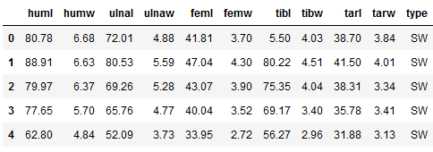
bird_df.isnull().sum()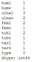
3 PyCaret - Classification
3.1 Setup
As a first step, I initialize the training environment. At the same time, the transformation pipeline is created. This setup function takes two parameters:
- the dataset
- the target variable
summary_preprocess = pycc.setup(bird_df, target = 'type')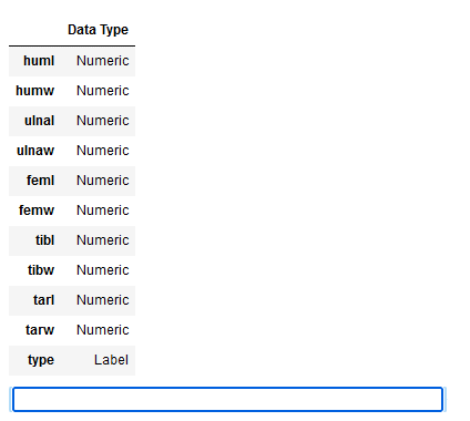
First we can check if the data types of all variables were recognized correctly. If this is the case, as here, we can press Enter.
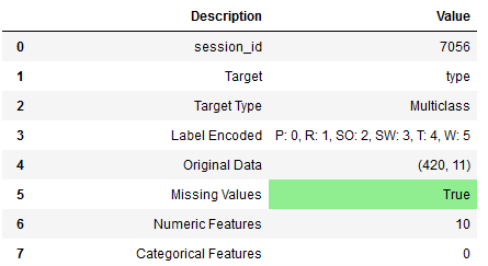
Now we get a detailed overview (only a part of it is shown here) of the initialized setup and the performed transformation steps of the pipeline.
Default Transformations:
- Missing Value Imputation
- Perfect Collinearity Removal
- One-Hot Encoding
- Train-Test Split
All transformations can be set individually in the setup function. See here: PyCaret Official - Preprocessing
These include:
- Data Preparation
- Missing Values
- Data Types
- Encoding
- Scale and Transform
- Feature Engineering
- Feature Selection and
- Other Parameters
Use these preprocessing and transformation parameters in the setup as needed for your present data set. In my example I leave it at the default settings.
Using the get_config function we can view the edited record.
x = pycc.get_config('X')
y = pycc.get_config('y')
trainX = pycc.get_config('X_train')
testX = pycc.get_config('X_test')
trainY = pycc.get_config('y_train')
testY = pycc.get_config('y_test')
x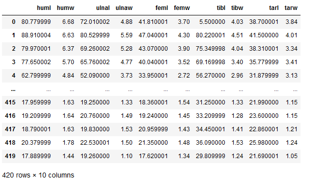
y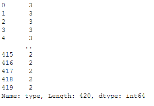
Here we see how the target variable ‘type’ has been recoded to apply machine learning algorithms. This step can also be seen in the summary_preprocess in line 4 (index 3).
If you want to get other values or information from the initiated setup here is a list of variables that can be retrieved using the get_config function: Variables accessible by get_config function
3.2 Compare Models
Now that all preprocessing steps are completed, we can check the performance of the classification algorithms available in PyCaret.
available_models = pycc.models()
available_models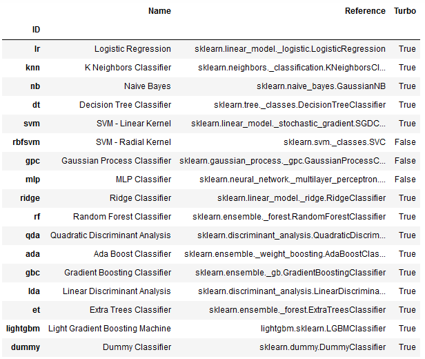
Now let’s compare these models:
best_clf = pycc.compare_models()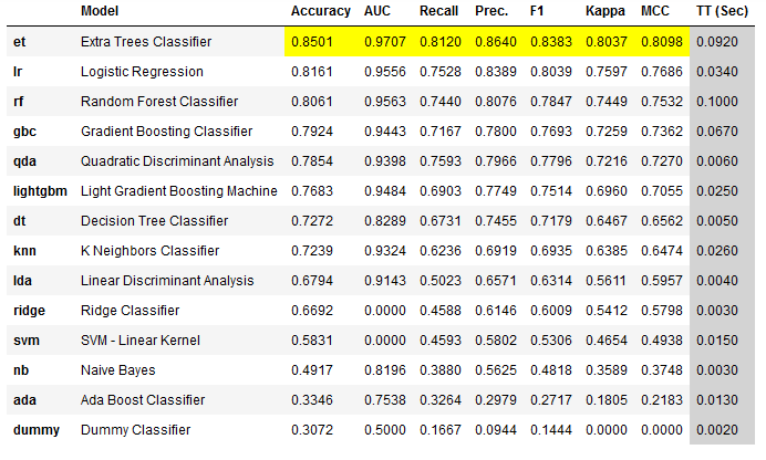
Another nice thing about this view is that the best values of each metric are highlighted in yellow. The Extra Trees Classifier achieved the highest value for almost every metric, so all highlighted fields are listed under this algorithm.
Let’s take a detailed look at the best model from the comparison:
print(best_clf)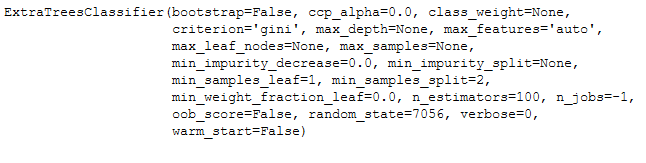
Changing the sort order
Of course, the highest Accuracy is not always the decisive metric, so sorting can also be done according to other evaluation metrics. Here, for example, the syntax to sort by AUC score:
best_clf_AUC = pycc.compare_models(sort = 'AUC')3.2.1 Comparison of Specific Models
Since model training can take different amounts of time, depending on the size of the data set, it is sometimes advisable to compare only certain models.
best_clf_specific = pycc.compare_models(include = ['ada', 'svm', 'nb'])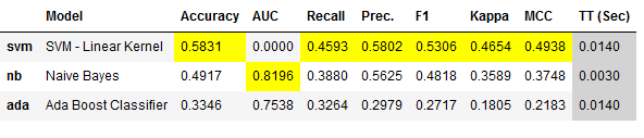
Exclusion of specific models:
Alternatively, certain models can simply be excluded from the performance comparison. See the following syntax:
best_clf_excl = pycc.compare_models(exclude = ['dummy', 'ridge'])3.2.2 Further Settings
In PyCaret you have the possibility to make further settings in the model comparison. These are:
The syntax to these settings would look like this:
best_clf_further_settings = pycc.compare_models(budget_time = 0.7,
                                                probability_threshold = 0.75,
                                                cross_validation=False)
3.3 Model Evaluation
Now that we have seen in our comparison (best_clf) that the Extra Trees Classifier has achieved the best values, I would like to go into the evaluation for this algorithm.
print(best_clf)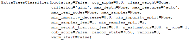
evaluation_best_clf = pycc.evaluate_model(best_clf)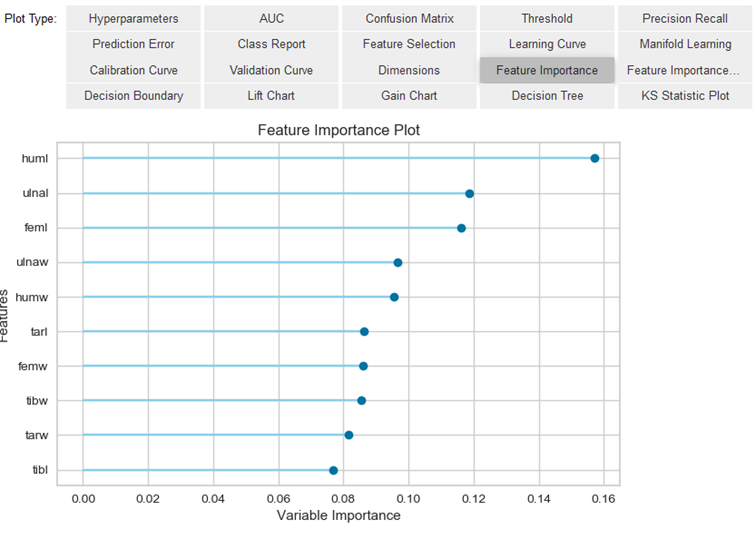
Since the evaluate_model function can only be used in notebooks, the plot_model function can also be used as an alternative.
pycc.plot_model(best_clf, plot = 'auc')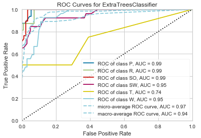
pycc.plot_model(best_clf, plot = 'confusion_matrix')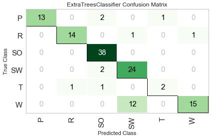
pycc.plot_model(best_clf,
                plot = 'confusion_matrix',
                plot_kwargs = {'percent' : True})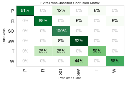
Saving image files
If you want to save the output graphics in PyCaret, you have to set the safe parameter to True. The syntax would look like this:
pycc.plot_model(best_clf,
                plot = 'confusion_matrix',
                plot_kwargs = {'percent' : True},
                save = True)
Here is an overview of possible graphics in PyCaret: Examples by module - Classification
3.4 Model Training
In comparing the classification algorithms, we saw that Extra Trees Classifier performed the best.
print(best_clf)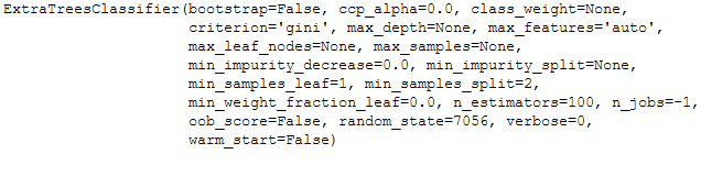
So we will do the model training with it as well. This is done in PyCaret with the create_model function, which also automatically includes cross-validation. Here I set the number of cross-validation runs to 5 (default = 10).
et_clf = pycc.create_model('et', fold = 5)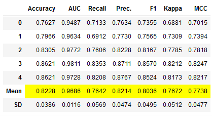
For some specific algorithms, the hyperparameters can be set specifically. Here is an example with the Decision Tree Classifier:
et_clf_custom_param = pycc.create_model('et',
                                        max_depth = 5)
Further Settings
As with model comparison, additional settings can be made during model training:
The syntax to these settings would look like this:
et_clf_further_settings = pycc.create_model('et',
                                            probability_threshold = 0.75,
                                            cross_validation=False)
Access performance metrics grid
The performance metrics are only displayed here, but not returned. However, they can be retrieved with the pull function.
et_clf_results = pycc.pull()
et_clf_results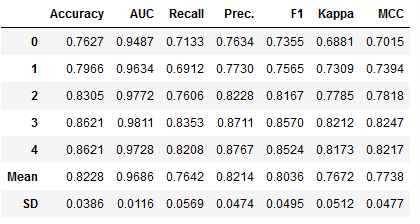
Filtered here according to the lines Mean and SD:
et_clf_results.loc[['Mean', 'SD']]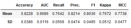
If you want to train multiple models or the same model with different configurations, you can do this with a for-loop. Have a look at this link: Train models in a loop
3.5 Model Optimization
There are several possibilities in PyCaret to further improve the performance of a model. I would like to present these in the following sections.
3.5.1 Tune the Model
If you want to tune the hyperparameters of the model, you have to use the tune_model function.
Since n_iter is set to 10 by default, I always like to increase this value as it improves the optimization. However, one must also mention here that the calculation time increases as a result.
et_clf_tuned = pycc.tune_model(et_clf, n_iter = 50)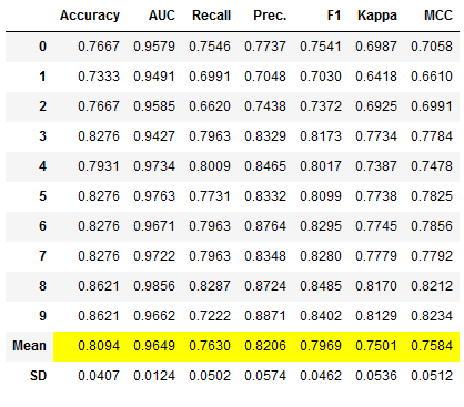
Access performance metrics grid
Again, the performance metrics are only displayed but not returned. Therefore we use the pull function again:
et_clf_tuned_results = pycc.pull()
et_clf_tuned_results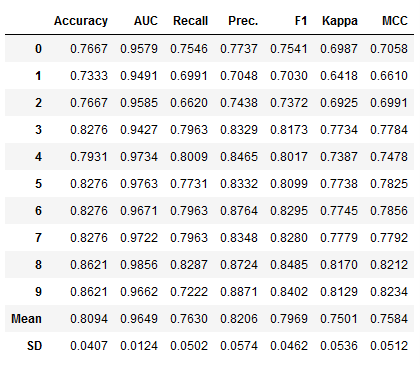
print(Color.BOLD +'Comparison of hyperparameters' + Color.END)
print()
print(Color.GREEN + Color.UNDERLINE + 'ExtraTreesClassifier:' + Color.END)
print()
print(et_clf)
print()
print(Color.RED + Color.UNDERLINE + 'ExtraTreesClassifier with Optimization:' + Color.END)
print()
print(et_clf_tuned)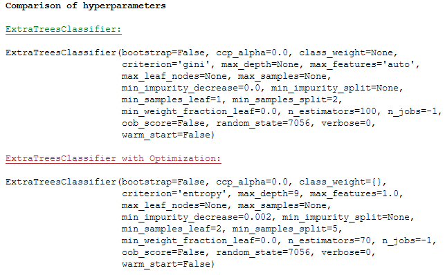
You can spend a lot of time optimizing ML algorithms, so there are also some parameters you can set in the tune_model function. These are among others:
- custom_grid
- search_library
- search_algorithm
- early_stopping
You can read about the other parameters here: pycaret.classification.tune_model()
3.5.2 Retrieve the Tuner
At this point I would like to go into more detail about one parameter: return_tuner=True
So far, we have only received the best model back from the tune_model function after optimizing the hyperparameters. But sometimes it is necessary to get back the tuner itself. This can be done with the additional argument return_tuner=True.
et_clf_tuned, et_clf_tuner = pycc.tune_model(et_clf,
                                             n_iter = 50,
                                             return_tuner=True)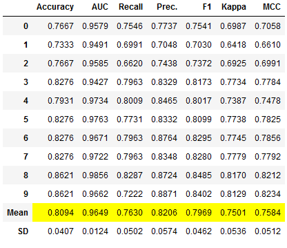
Here it is:
et_clf_tuner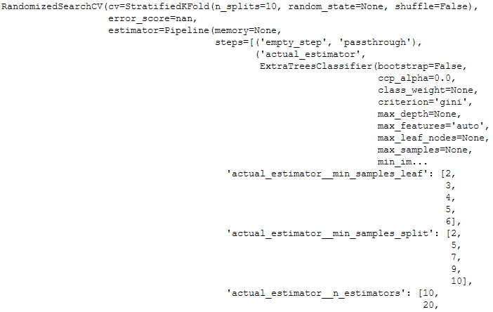
3.5.3 Automatically Choose Better
A tuned model does not always deliver better results. See the performance overview of the two models in the comparison:
print(Color.BOLD +'Comparison of performance metrics' + Color.END)
print()
print(Color.GREEN + Color.UNDERLINE + 'ExtraTreesClassifier:' + Color.END)
print()
print(et_clf_results.loc[['Mean']])
print()
print(Color.RED + Color.UNDERLINE + 'ExtraTreesClassifier with Optimization:' + Color.END)
print()
print(et_clf_tuned_results.loc[['Mean']])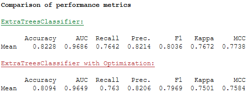
To prevent this from accidentally becoming a problem, there is the choose_better parameter. If this is set to True, an improved model is always returned. Even if the optimization of the hyperparameters does not result in an improvement, the original model is returned instead of a worse model as was the case above.
et_clf_tuned_better, \
et_clf_tuned_better_tuner = pycc.tune_model(et_clf,n_iter = 50,
                                            return_tuner=True,
                                            choose_better = True)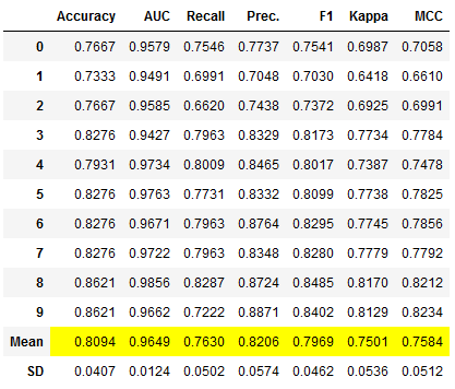
Please do not be confused by the performance overview. This shows the metrics for the best model that the tuner has created. If the performance cannot be increased, the worse model is not returned by the tuner but the old model is used (now also stored under the object et_clf_tuned_better).
The grid of performance indicators can again be assigned to an object by pull:
et_clf_tuned_better_results = pycc.pull()If someone does not like this approach, they are welcome to continue with the old model (et_clf).
3.5.4 ensemble_models
Another way to improve the existing model is to create an ensemble. For this we have two options here:
By default, PyCaret always uses 10 estimators for these two methods. However, I want more to be used right away, so I specify this parameter for both methods right away.
I will train new models for both methods and then compare performance.
Method: Bagging:
# Train the bagged Model
et_clf_bagged = pycc.ensemble_model(et_clf,
                                    method = 'Bagging',
                                    fold = 5,
                                    n_estimators = 100)

# Obtaining the performance overview
et_clf_bagged_results = pycc.pull()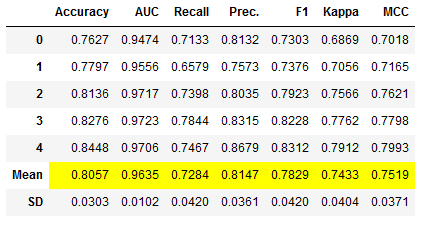
Method: Boosting:
# Train the boosted Model
et_clf_boosted = pycc.ensemble_model(et_clf,
                                     method = 'Boosting',
                                     fold = 5,
                                     n_estimators = 100)

# Obtaining the performance overview
et_clf_boosted_results = pycc.pull()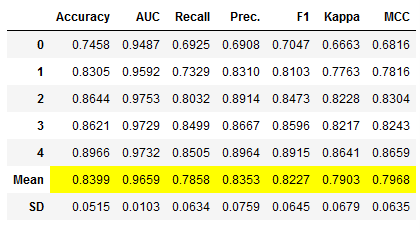
Overview of the performance metrics:
print(Color.BOLD +'Comparison of performance metrics' + Color.END)
print()
print('ExtraTreesClassifier:')
print()
print(et_clf_results.loc[['Mean']])
print()
print('ExtraTreesClassifier with Optimization:')
print()
print(et_clf_tuned_results.loc[['Mean']])
print()
print('ExtraTreesClassifier bagged:')
print()
print(et_clf_bagged_results.loc[['Mean']])
print()
print('ExtraTreesClassifier boosted:')
print()
print(et_clf_boosted_results.loc[['Mean']])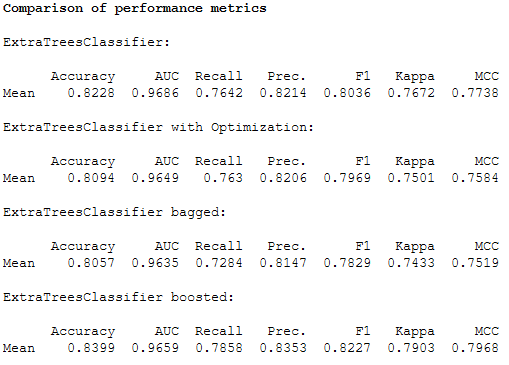
Since this is a little hard to read, I always quite like to create the following overview:
et_clf_results_df = et_clf_results.loc[['Mean']]
et_clf_tuned_results_df = et_clf_tuned_results.loc[['Mean']]
et_clf_bagged_results_df = et_clf_bagged_results.loc[['Mean']]
et_clf_boosted_results_df = et_clf_boosted_results.loc[['Mean']]

comparison_df = pd.concat([et_clf_results_df,
                          et_clf_tuned_results_df,
                          et_clf_bagged_results_df,
                          et_clf_boosted_results_df]).reset_index()

comparison_df = comparison_df.drop('index', axis=1)
comparison_df.insert(0, "Model", ['et_clf', 'et_clf_tuned',
                                  'et_clf_bagged', 'et_clf_boosted'])

comparison_df.style.highlight_max(color = 'lightgreen', axis = 0)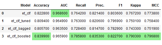
The overview shows us that the et_clf_boosted model performs best.
As with the tune_model function, there is also the choose_better = True parameter here. Use this one if you like.
3.5.5 blend_models
Another way I would like to introduce to improve performance is to use voting classifiers.
I have also written a post about this topic before see here: Ensemble Modeling - Voting
# Training of multiple models
lr_clf_voting = pycc.create_model('lr', fold = 5)
dt_clf_voting = pycc.create_model('dt', fold = 5)
et_clf_voting = pycc.create_model('et', fold = 5)

voting_clf = pycc.blend_models([lr_clf_voting,
                                dt_clf_voting,
                                et_clf_voting])

# Obtaining the performance overview
voting_clf_results = pycc.pull()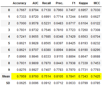
Dynamic input estimators
The list of input estimators can also be created automatically using the compare_models function. We have used this function in chapter 3.2. Here the N best models are used as input list.
# Training of N best models
voting_clf_dynamic = pycc.blend_models(pycc.compare_models(n_select = 3))
# Obtaining the performance overview
voting_clf_dynamic_results = pycc.pull()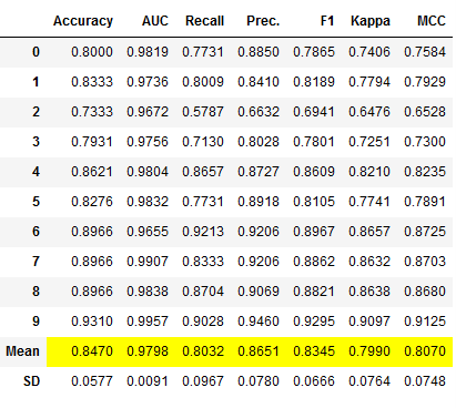
Here you can see which estimator was finally used:
voting_clf_dynamic.estimators_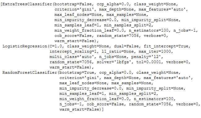
Here is a performance overview again. I have left out the models that have not brought any improvement, so that it remains clear.
et_clf_results_df = et_clf_results.loc[['Mean']]
et_clf_boosted_results_df = et_clf_boosted_results.loc[['Mean']]
voting_clf_results_df = voting_clf_results.loc[['Mean']]
voting_clf_dynamic_results_df = voting_clf_dynamic_results.loc[['Mean']]

comparison_df2 = pd.concat([et_clf_results_df,
                            et_clf_boosted_results_df,
                            voting_clf_results_df,
                            voting_clf_dynamic_results_df]).reset_index()

comparison_df2 = comparison_df2.drop('index', axis=1)
comparison_df2.insert(0, "Model", ['et_clf',
                                   'et_clf_boosted',
                                   'voting_clf',
                                   'voting_clf_dynamic'])

comparison_df2.style.highlight_max(color = 'lightgreen', axis = 0)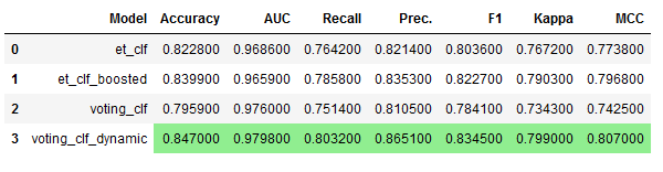
We have managed to find an even better model!
With blend_models, there are other parameters that could improve performance. These are:
As with the tune_model function, there is also the choose_better = True parameter here. Use this one if you like.
3.5.6 stack_models
Which function should not be missing under the chapter Model Optimization and is also available in PyCaret is the stack_models function.
I have already written a post about this topic for those who want to learn more about this method: Ensemble Modeling - Stacking
The procedure and syntax is almost identical to the blend_models function.
# Training of multiple models
lr_clf_stacked = pycc.create_model('lr', fold = 5)
dt_clf_stacked = pycc.create_model('dt', fold = 5)
et_clf_stacked = pycc.create_model('et', fold = 5)

stacked_clf = pycc.stack_models([lr_clf_stacked,
                                dt_clf_stacked,
                                et_clf_stacked])

# Obtaining the performance overview
stacked_clf_results = pycc.pull()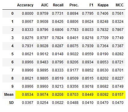
Dynamic input estimators
As with the blend_models function, the list of input estimators can also be created automatically with the compare_models function. Here again the N best models are used as input list.
# Training of N best models
stacked_clf_dynamic = pycc.stack_models(pycc.compare_models(n_select = 3))
# Obtaining the performance overview
stacked_clf_dynamic_results = pycc.pull()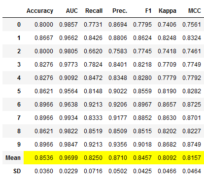
And here again the overview of the estimators that were used.
stacked_clf_dynamic.estimators_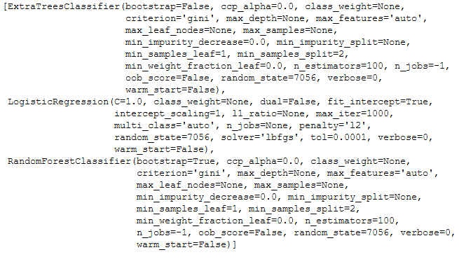
Let’s take another look at the performance overviews. Again, I have only listed the relevant ones and omitted the overviews for less performant algorithms.
et_clf_results_df = et_clf_results.loc[['Mean']]
voting_clf_dynamic_results_df = voting_clf_dynamic_results.loc[['Mean']]
stacked_clf_results_df = stacked_clf_results.loc[['Mean']]
stacked_clf_dynamic_results_df = stacked_clf_dynamic_results.loc[['Mean']]

comparison_df3 = pd.concat([et_clf_results_df,
                            voting_clf_dynamic_results_df,
                            stacked_clf_results_df,
                            stacked_clf_dynamic_results_df]).reset_index()

comparison_df3 = comparison_df3.drop('index', axis=1)
comparison_df3.insert(0, "Model", ['et_clf',
                                   'voting_clf_dynamic',
                                   'stacked_clf',
                                   'stacked_clf_dynamic'])

comparison_df3.style.highlight_max(color = 'lightgreen', axis = 0)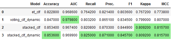
We were able to improve performance once again.
With stack_models, there are other parameters that could improve performance. These are:
As with the tune_model function, there is also the choose_better = True parameter here. Use this one if you like.
3.5.7 Further Methods
There are two more methods in PyCaret that I would like to mention briefly here:
Please read the documentation and decide for yourself if these methods help you.
3.6 Model Evaluation after Training
I have already discussed the evaluation possibilities via PyCaret in chapter 3.3. Here we only looked at how well the performance of the algorithms fit the training part of our data to get an impression of which model might fit best.
In the following I will do this again with a trained model for the test part. For this I use the model created in chapter 3.5.6 (stacked_clf_dynamic), because this gave the best performance values during the model optimization.
type(stacked_clf_dynamic)
pycc.plot_model(stacked_clf_dynamic, plot = 'auc', scale = 2)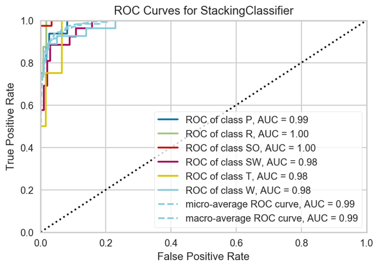
Use train data
If you want to know what performance the trained model has on the training data, you can use_train_data = True. Here is an example:
pycc.plot_model(stacked_clf_dynamic, plot = 'auc',
                scale = 2,
                use_train_data = True)
Saving image files
If you want to save the output graphics in PyCaret, you have to set the safe parameter to True. The syntax would look like this:
pycc.plot_model(stacked_clf_dynamic, plot = 'auc',
                scale = 2,
                save = True)
Here is an overview of possible graphics in PyCaret: Examples by module
3.7 Model Predictions
Now we come to the part where we make predictions with our trained algorithm. Here we use the following model, since it has shown the best validation values:
type(stacked_clf_dynamic)
3.7.1 On testX
As a reminder, here is the test part of our data set, which was generated by the Train-Test Split in the setup function (see chapter 3.1).
testX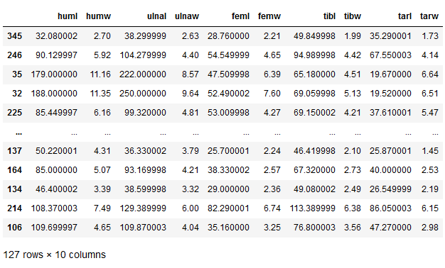
# Make model predictions on testX
stacked_clf_dynamic_pred = pycc.predict_model(stacked_clf_dynamic)
stacked_clf_dynamic_pred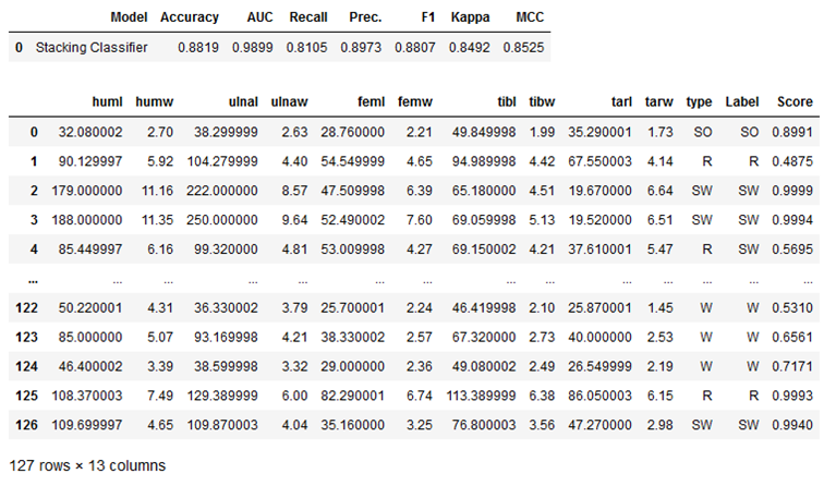
As we can see, three more columns have been added to the testX part:
- type -> These are the true labels in their original form (not recoded)
- Label -> these are the predicted labels (also not recoded)
- Score -> These are the score values for the predicted labels
# Obtaining the performance overview
stacked_clf_dynamic_pred_results = pycc.pull()
stacked_clf_dynamic_pred_results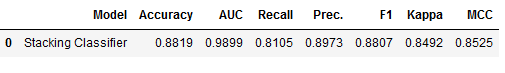
If we look at the performance values for the prediction, we see that with an accuracy of over 88%, this is even better than that achieved during model training:
stacked_clf_dynamic_results_df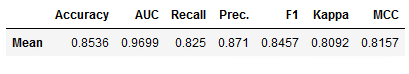
The variation comes from the fact that we used cross-validation in model training for this algorithm. Keep this in mind when reporting results to your supervisor or client.
3.7.2 On unseen data
Now is the time to make predictions about unseen data. I have created my own data set for this purpose:
unseen_df = pd.DataFrame(np.array([[165.00,11.45,156.00,8.68,80.25,7.85,143.00,8.25,86.61,6.63],
                                   [63.48,4.03,77.33,3.65,26.84,2.31,48.82,2.51,22.91,1.7],
                                   [13.52,1.28,17.88,1.07,15.1,1.05,25.14,1.23,17.81,0.69],
                                   [20.25,2.35,25.14,1.76,20.17,1.37,27.67,1.41,15.68,1.55],
                                   [62.49,4.75,69.66,3.99,57.3,4.6,77.6,4.26,60.31,3.86],
                                   [31.72,2.64,40,1.99,20.36,1.59,32.21,1.62,17.72,1.52],
                                   [28.66,2.48,33.24,2.02,29.33,2.26,50.64,2.05,35.99,1.85],
                                   [68.15,3.84,72.31,3.42,24.23,1.9,50.26,2.13,29.16,2.05]]),
                         columns=['huml', 'humw', 'ulnal', 'ulnaw', 'feml',
                                  'femw', 'tibl', 'tibw', 'tarl', 'tarw'])


unseen_df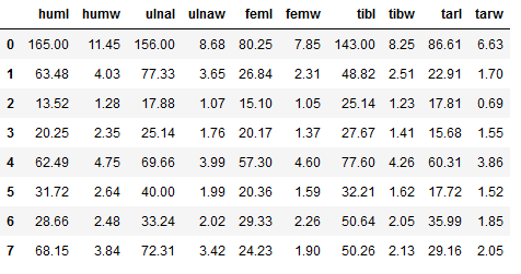
Of course, the data set must contain the same number of variables as it did during setup and model training.
If you use the predict_model function on new (unseen) data, you have to pass the parameter data = ‘name_of_the_new_data’ to the function. Furthermore I use raw_score = True to see which scores are calculated for the respective classes.
# Make model predictions on unseen data
stacked_clf_dynamic_pred_unseen = pycc.predict_model(stacked_clf_dynamic,
                                                     raw_score = True,
                                                     data = unseen_df)

stacked_clf_dynamic_pred_unseen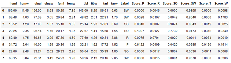
Done! We made our first prediction with the model we created.
Below I show again the effect of the raw_score = True setting. To do this, I selected the newly generated columns:
stacked_clf_dynamic_pred_unseen.loc[:,'Label' : 'Score_W']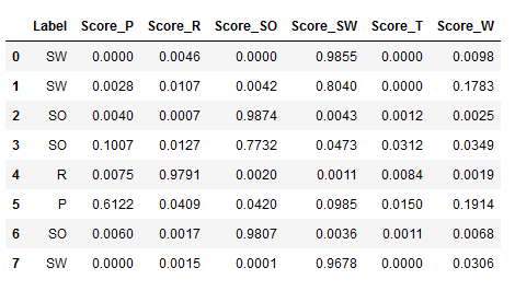
The column ‘Label’ shows again the predicted labels. After that come the score values for the respective classes.
So the model says with a probability of over 98% that the observation from line 1 belongs to the class ‘SW’.
3.8 Model Finalization
Last but not least, we finalize our model. Here, the final model is trained again on both the trainX part and the testX part. No more changes are made to the model parameters.
stacked_clf_dynamic_final = pycc.finalize_model(stacked_clf_dynamic)
stacked_clf_dynamic_final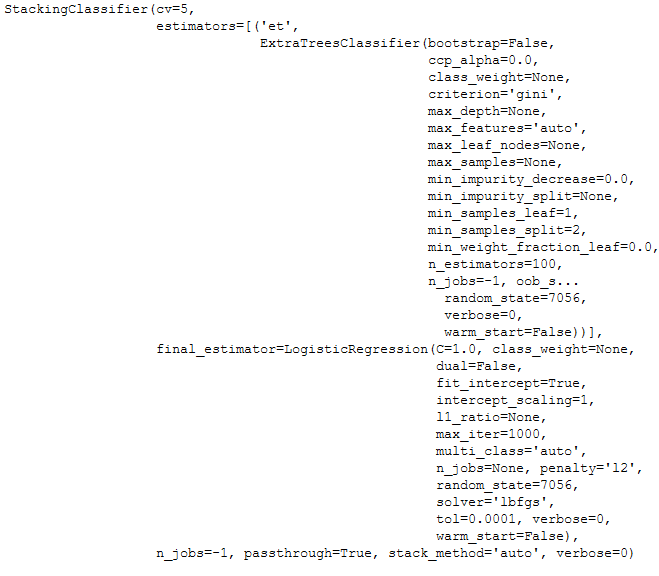
3.9 Saving the Pipeline & Model
To be able to use the created pipeline and the trained model in another place, we have to save it as a last step.
pycc.save_model(stacked_clf_dynamic_final,
                'stacked_clf_dynamic_final_pipeline')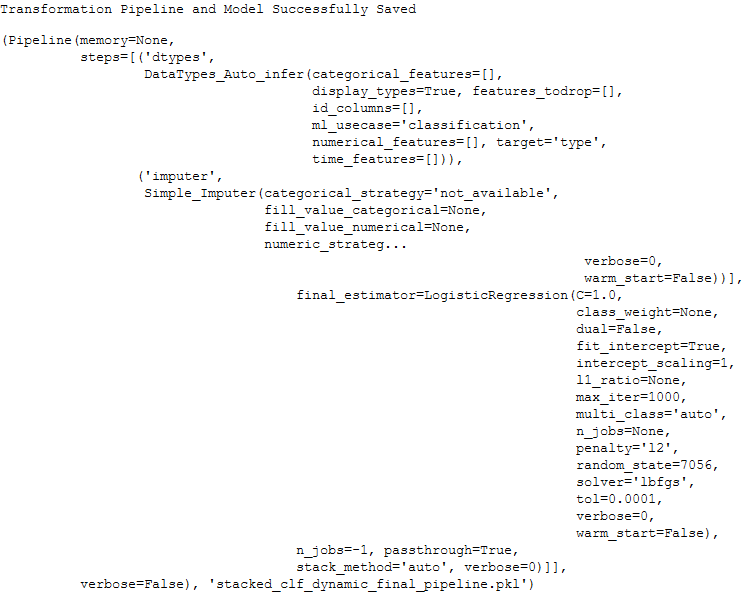
Reload a Pipeline
Let’s review this as well:
pipeline_reload = pycc.load_model('stacked_clf_dynamic_final_pipeline')
Ready for new predictions
unseen_df2 = pd.DataFrame(np.array([[34.07,3.26,41.34,2.62,24.25,2.3,36.35,2.13,24.69,2.12]]),
                          columns=['huml', 'humw', 'ulnal', 'ulnaw', 'feml',
                                   'femw', 'tibl', 'tibw', 'tarl', 'tarw'])


unseen_df2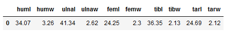
pipeline_reload_pred_unseen2 = pycc.predict_model(pipeline_reload,
                                                  raw_score = True,
                                                  data = unseen_df2)

pipeline_reload_pred_unseen2
Works !
4 Conclusion
In this post I showed how to use PyCaret to solve a classification problem and demonstrated the power behind this AutoML library.
With PyCaret you have the possibility to quickly and easily run different scenarios in model training and find the best fitting algorithm for your problem.
Thanks also to the PyCaret team for giving me quick feedback on my questions.
Limitations
In this post, I applied very few data pre-processing steps. Scaling or feature engineering, for example, could have increased the performance even more.