1 Introduction

Some time ago I had written the post The Data Science Process (CRISP-DM), which was about the correct development of Machine Learning algorithms. As you have seen here, this is quite a time-consuming matter if done correctly.
In order to quickly check which algorithm fits the data best, it is recommended to use machine learning pipelines. Once you have found a promising algorithm, you can start fine tuning with it and go through the process as described here.
For this post the dataset bird from the statistic platform “Kaggle” was used. You can download it from my “GitHub Repository”.
2 Loading the libraries and classes
import pandas as pd
import numpy as np

from sklearn.model_selection import train_test_split


from sklearn.preprocessing import StandardScaler
from sklearn.preprocessing import MinMaxScaler
from sklearn.preprocessing import RobustScaler

from sklearn.decomposition import PCA


from sklearn.linear_model import LogisticRegression
from sklearn.svm import SVC
from sklearn.neighbors import KNeighborsClassifier
from sklearn.tree import DecisionTreeClassifier
from sklearn.ensemble import RandomForestClassifier

from sklearn.pipeline import Pipeline

from sklearn.metrics import accuracy_score
class Color:
PURPLE = '\033[95m'
CYAN = '\033[96m'
DARKCYAN = '\033[36m'
BLUE = '\033[94m'
GREEN = '\033[92m'
YELLOW = '\033[93m'
RED = '\033[91m'
BOLD = '\033[1m'
UNDERLINE = '\033[4m'
END = '\033[0m'3 Loading the data
bird_df = pd.read_csv('bird.csv').dropna()
bird_df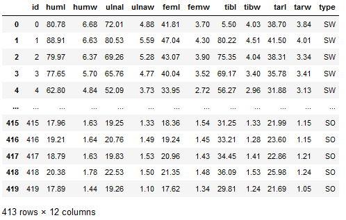
Description of predictors:
- Length and Diameter of Humerus
- Length and Diameter of Ulna
- Length and Diameter of Femur
- Length and Diameter of Tibiotarsus
- Length and Diameter of Tarsometatarsus
bird_df['type'].value_counts()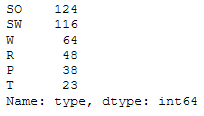
Description of the target variable:
- SW: Swimming Birds
- W: Wading Birds
- T: Terrestrial Birds
- R: Raptors
- P: Scansorial Birds
- SO: Singing Birds
bird_df['type'].nunique()
x = bird_df.drop(['type', 'id'], axis=1)
y = bird_df['type']

trainX, testX, trainY, testY = train_test_split(x, y, test_size = 0.2)
4 ML Pipelines
4.1 A simple Pipeline
Let’s start with a simple pipeline.
In the following, I would like to perform a classification of bird species using Logistic Regression. For this purpose, the data should be scaled beforehand using the StandardScaler of scikit-learn.
Creation of the pipeline:
pipe_lr = Pipeline([
    ('ss', StandardScaler()),
    ('lr', LogisticRegression())
    ])
Fit and Evaluate the Pipeline:
pipe_lr.fit(trainX, trainY)y_pred = pipe_lr.predict(testX)
print('Test Accuracy: {:.2f}'.format(accuracy_score(testY, y_pred)))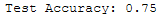
OK, .75% not bad. Let’s see if we can improve the result by choosing a different scaler.
4.2 Determination of the best Scaler
4.2.1 Creation of the Pipeline
pipe_lr_wo = Pipeline([
    ('lr', LogisticRegression())
    ])

pipe_lr_ss = Pipeline([
    ('ss', StandardScaler()),
    ('lr', LogisticRegression())
    ])

pipe_lr_mms = Pipeline([
    ('mms', MinMaxScaler()),
    ('lr', LogisticRegression())
    ])

pipe_lr_rs = Pipeline([
    ('rs', RobustScaler()),
    ('lr', LogisticRegression())
    ])
4.2.2 Creation of a Pipeline Dictionary
To be able to present the later results better, I always create a suitable dictionary at this point.
pipe_dic = {
    0: 'LogReg wo scaler',
    1: 'LogReg with StandardScaler',
    2: 'LogReg with MinMaxScaler',
    3: 'LogReg with RobustScaler',
    }

pipe_dic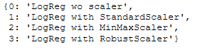
4.2.3 Fit the Pipeline
To be able to fit the pipelines, I first need to group the pipelines into a list:
pipelines = [pipe_lr_wo, pipe_lr_ss, pipe_lr_mms, pipe_lr_rs]Now we are going to fit the created pipelines:
for pipe in pipelines:
    pipe.fit(trainX, trainY)
4.2.4 Evaluate the Pipeline
for idx, val in enumerate(pipelines):
    print('%s pipeline Test Accuracy: %.2f' % (pipe_dic[idx], accuracy_score(testY, val.predict(testX))))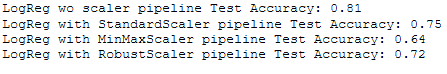
We can also use the .score function:
for idx, val in enumerate(pipelines):
    print('%s pipeline Test Accuracy: %.2f' % (pipe_dic[idx], val.score(testX, testY)))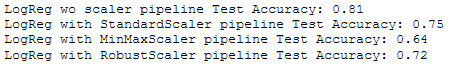
I always like to have the results displayed in a dataframe so I can sort and filter:
result = []

for idx, val in enumerate(pipelines):
    result.append(accuracy_score(testY, val.predict(testX)))


result_df = pd.DataFrame(list(pipe_dic.items()),columns = ['Idx','Estimator'])

# Add Test Accuracy to result_df
result_df['Test_Accuracy'] = result
# print result_df
result_df 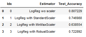
Let’s take a look at our best model:
best_model = result_df.sort_values(by='Test_Accuracy', ascending=False)
best_model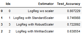
print(best_model['Estimator'].iloc[0] +
      ' Classifier has the best Test Accuracy of ' +
      str(round(best_model['Test_Accuracy'].iloc[0], 2)) + '%')
Or the print statement still a little bit spiffed up:
print(Color.RED + best_model['Estimator'].iloc[0] + Color.END +
      ' Classifier has the best Test Accuracy of ' +
      Color.GREEN + Color.BOLD + str(round(best_model['Test_Accuracy'].iloc[0], 2)) + '%')
4.3 Determination of the best Estimator
Let’s try this time with different estimators to improve the result.
4.3.1 Creation of the Pipeline
pipe_lr = Pipeline([
    ('ss1', StandardScaler()),
    ('lr', LogisticRegression())
    ])

pipe_svm_lin = Pipeline([
    ('ss2', StandardScaler()),
    ('svm_lin', SVC(kernel='linear'))
    ])

pipe_svm_sig = Pipeline([
    ('ss3', StandardScaler()),
    ('svm_sig', SVC(kernel='sigmoid'))
    ])


pipe_knn = Pipeline([
    ('ss4', StandardScaler()),
    ('knn', KNeighborsClassifier(n_neighbors=7))
    ])

pipe_dt = Pipeline([
    ('ss5', StandardScaler()),
    ('dt', DecisionTreeClassifier())
    ])

pipe_rf = Pipeline([
    ('ss6', StandardScaler()),
    ('rf', RandomForestClassifier(n_estimators=100))
    ])
4.3.2 Creation of a Pipeline Dictionary
pipe_dic = {
    0: 'lr',
    1: 'svm_lin',
    2: 'svm_sig',
    3: 'knn',
    4: 'dt',
    5: 'rf'
    }

pipe_dic
4.3.3 Fit the Pipeline
pipelines = [pipe_lr, pipe_svm_lin, pipe_svm_sig, pipe_knn, pipe_dt, pipe_rf]for pipe in pipelines:
pipe.fit(trainX, trainY)4.3.4 Evaluate the Pipeline
for idx, val in enumerate(pipelines):
    print('%s pipeline Test Accuracy: %.2f' % (pipe_dic[idx], accuracy_score(testY, val.predict(testX))))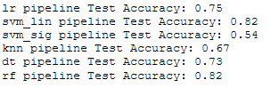
result = []

for idx, val in enumerate(pipelines):
    result.append(accuracy_score(testY, val.predict(testX)))


result_df = pd.DataFrame(list(pipe_dic.items()),columns = ['Idx','Estimator'])

# Add Test Accuracy to result_df
result_df['Test_Accuracy'] = result
# print result_df
result_df 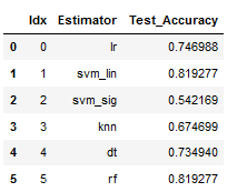
best_model = result_df.sort_values(by='Test_Accuracy', ascending=False)
best_model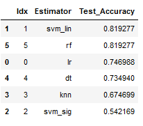
print(Color.RED + best_model['Estimator'].iloc[0] + Color.END +
      ' Classifier has the best Test Accuracy of ' +
      Color.GREEN + Color.BOLD + str(round(best_model['Test_Accuracy'].iloc[0], 2)) + '%')
Done. The linear support vector classifier has improved the accuracy.
4.4 ML Pipelines with further Components
At this point you can now play wonderfully. You can add different scalers to the Estimators or even try including a PCA.
I use the same pipeline as in the previous example and add a PCA with n_components=2 to the estimators.
pipe_lr = Pipeline([
    ('ss1', StandardScaler()),
    ('pca1', PCA(n_components=2)),
    ('lr', LogisticRegression())
    ])

pipe_svm_lin = Pipeline([
    ('ss2', StandardScaler()),
    ('pca2', PCA(n_components=2)),
    ('svm_lin', SVC(kernel='linear'))
    ])

pipe_svm_sig = Pipeline([
    ('ss3', StandardScaler()),
    ('pca3', PCA(n_components=2)),
    ('svm_sig', SVC(kernel='sigmoid'))
    ])


pipe_knn = Pipeline([
    ('ss4', StandardScaler()),
    ('pca4', PCA(n_components=2)),
    ('knn', KNeighborsClassifier(n_neighbors=7))
    ])

pipe_dt = Pipeline([
    ('ss5', StandardScaler()),
    ('pca5', PCA(n_components=2)),
    ('dt', DecisionTreeClassifier())
    ])

pipe_rf = Pipeline([
    ('ss6', StandardScaler()),
    ('pca6', PCA(n_components=2)),
    ('rf', RandomForestClassifier(n_estimators=100))
    ])
pipe_dic = {
0: 'lr',
1: 'svm_lin',
2: 'svm_sig',
3: 'knn',
4: 'dt',
5: 'rf'
}pipelines = [pipe_lr, pipe_svm_lin, pipe_svm_sig, pipe_knn, pipe_dt, pipe_rf]for pipe in pipelines:
pipe.fit(trainX, trainY)for idx, val in enumerate(pipelines):
print('%s pipeline Test Accuracy: %.2f' % (pipe_dic[idx], accuracy_score(testY, val.predict(testX))))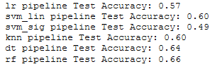
result = []

for idx, val in enumerate(pipelines):
    result.append(accuracy_score(testY, val.predict(testX)))


result_df = pd.DataFrame(list(pipe_dic.items()),columns = ['Idx','Estimator'])

# Add Test Accuracy to result_df
result_df['Test_Accuracy'] = result
# print result_df
result_df 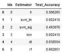
best_model = result_df.sort_values(by='Test_Accuracy', ascending=False)
best_model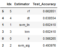
print(Color.RED + best_model['Estimator'].iloc[0] + Color.END +
      ' Classifier has the best Test Accuracy of ' +
      Color.GREEN + Color.BOLD + str(round(best_model['Test_Accuracy'].iloc[0], 2)) + '%')
The use of a PCA has not worked out any improvement. We can therefore fall back on the linear Support Vector Classifier at this point and try to improve the result again with Fine Tuning.
5 Conclusion
In this post, I showed how to use machine learning pipelines to quickly and efficiently run different scenarios to get a first impression of which algorithm fits my data best.