1 Introduction
So far we have dealt very intensively with the use of different classification algorithms. Now let’s come to some ensemble methods. Ensemble learning is a machine learning paradigm where multiple models (often called “weak learners”) are trained to solve the same problem and combined to get better results.
There are three most common types of ensembles:
- Bagging
- Boosting
- Stacking
In this post we will start with bagging, and then move on to boosting and stacking in separate publications.
For this post the dataset Bank Data from the platform “UCI Machine Learning Repository” was used. You can download it from my “GitHub Repository”.
2 Background Information on Bagging
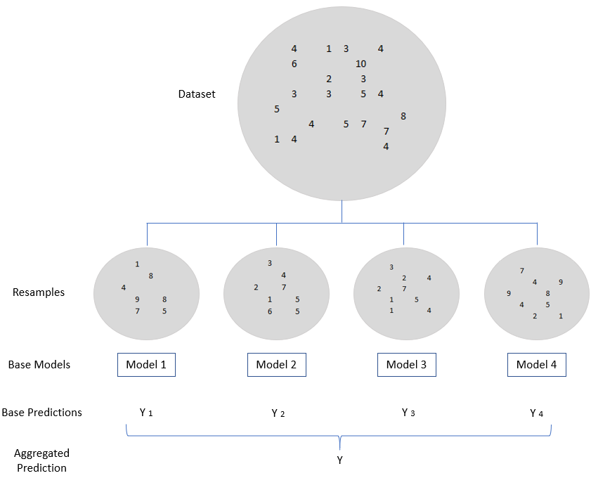
The term bagging is derived from a technique calles bootstrap aggregation. In a nutshell: The bootstrap method refers to random sampling with replacement (please see figure below). Several small data records (resamples) are removed from an existing data record. It doesn’t matter whether an observation is taken out twice or not. With the help of these resamples, individual models are calculated and ultimately combined to form an aggregated prediction.
3 Loading the libraries and the data
import numpy as np
import pandas as pd
import matplotlib.pyplot as plt

from sklearn.model_selection import train_test_split

from sklearn.tree import DecisionTreeClassifier
from sklearn.ensemble import BaggingClassifier

from sklearn.metrics import accuracy_score


from sklearn.ensemble import RandomForestClassifier

from sklearn.model_selection import StratifiedKFold
from sklearn.model_selection import cross_val_score

from sklearn.model_selection import RandomizedSearchCV
bank = pd.read_csv("bank.csv", sep=";")
bank.head()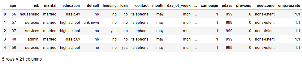
The data set before us contains information about whether a customer has signed a contract or not.
bank['y'].value_counts().T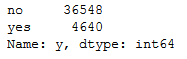
Let’s see how well we can predict that in the end.
4 Data pre-processing
Here we convert all categorical variables into numerical. If you want to know exactly how it works look at these two posts of mine:
safe_y = bank[['y']]

col_to_exclude = ['y']
bank = bank.drop(col_to_exclude, axis=1)
#Just select the categorical variables
cat_col = ['object']
cat_columns = list(bank.select_dtypes(include=cat_col).columns)
cat_data = bank[cat_columns]
cat_vars = cat_data.columns
#Create dummy variables for each cat. variable
for var in cat_vars:
cat_list = pd.get_dummies(bank[var], prefix=var)
bank=bank.join(cat_list)
data_vars=bank.columns.values.tolist()
to_keep=[i for i in data_vars if i not in cat_vars]
#Create final dataframe
bank_final=bank[to_keep]
bank_final.columns.values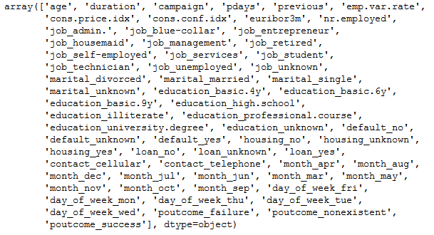
bank = pd.concat([bank_final, safe_y], axis=1)
bank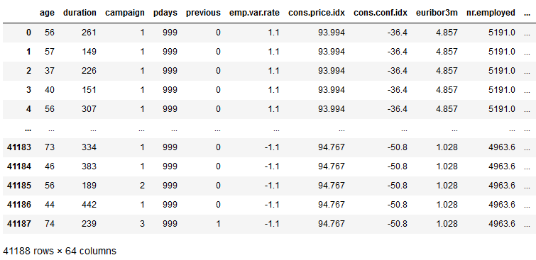
Let’s check for missing values:
def missing_values_table(df):
        # Total missing values
        mis_val = df.isnull().sum()

        # Percentage of missing values
        mis_val_percent = 100 * df.isnull().sum() / len(df)

        # Make a table with the results
        mis_val_table = pd.concat([mis_val, mis_val_percent], axis=1)

        # Rename the columns
        mis_val_table_ren_columns = mis_val_table.rename(
        columns = {0 : 'Missing Values', 1 : '% of Total Values'})

        # Sort the table by percentage of missing descending
        mis_val_table_ren_columns = mis_val_table_ren_columns[
            mis_val_table_ren_columns.iloc[:,1] != 0].sort_values(
        '% of Total Values', ascending=False).round(1)

        # Print some summary information
        print ("Your selected dataframe has " + str(df.shape[1]) + " columns.\n"
            "There are " + str(mis_val_table_ren_columns.shape[0]) +
              " columns that have missing values.")

        # Return the dataframe with missing information
        return mis_val_table_ren_columns
missing_values_table(bank)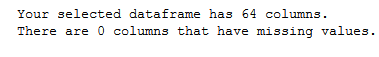
No missing values. Perfect! Now let’s split the dataframe for further processing.
x = bank.drop('y', axis=1)
y = bank['y']

trainX, testX, trainY, testY = train_test_split(x, y, test_size = 0.2)
5 Decision Tree Classifier
Let’s see how well the Decision Tree Classifier works with our data set.
dt_params = {
    'criterion': 'entropy',
    'random_state': 11
}
dt = DecisionTreeClassifier(**dt_params)
dt.fit(trainX, trainY)
dt_preds_train = dt.predict(trainX)
dt_preds_test = dt.predict(testX)
print('Decision Tree:\n> Accuracy on training data = {:.4f}\n> Accuracy on test data = {:.4f}'.format(
accuracy_score(trainY, dt_preds_train),
accuracy_score(testY, dt_preds_test)
))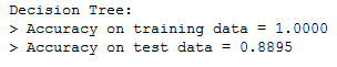
88% accuracy on the test set. Not bad. Let’s try to improve this result with an ensemble method.
6 Bagging Classifier
bc_params = {
    'base_estimator': dt,
    'n_estimators': 50,
    'max_samples': 0.5,
    'random_state': 11,
    'n_jobs': -1
}
bc = BaggingClassifier(**bc_params)
bc.fit(trainX, trainY)
bc_preds_train = bc.predict(trainX)
bc_preds_test = bc.predict(testX)
print('Bagging Classifier:\n> Accuracy on training data = {:.4f}\n> Accuracy on test data = {:.4f}'.format(
accuracy_score(trainY, bc_preds_train),
accuracy_score(testY, bc_preds_test)
))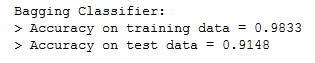
Perfect. We could improve the result to 91% accuracy.
7 Random Forest Classifier
Random Forest is probably one of the best-known algorithms worldwide and also builds on the bootstrapping method. Random Forest not only bootstrapping the data points in the overall training dataset, but also bootstrapping the features available for each tree to split on.
7.1 Train the Random Forest Classifier
rf_params = {
    'n_estimators': 100,
    'criterion': 'entropy',
    'max_features': 0.5,
    'min_samples_leaf': 10,
    'random_state': 11,
    'n_jobs': -1
}
rf = RandomForestClassifier(**rf_params)
rf.fit(trainX, trainY)
rf_preds_train = rf.predict(trainX)
rf_preds_test = rf.predict(testX)
print('Random Forest Classifier:\n> Accuracy on training data = {:.4f}\n> Accuracy on test data = {:.4f}'.format(
accuracy_score(trainY, rf_preds_train),
accuracy_score(testY, rf_preds_test)
))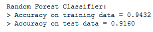
As we can see, we were able to increase the model predictive power again.
7.2 Evaluate the Forest Classifier
7.2.1 StratifiedKFold
The StratifiedKFold class in scikit-learn implements a combination of the cross-validation and sampling together in one class.
x = bank.drop('y', axis=1).values
y = bank['y'].values

skf = StratifiedKFold(n_splits=10)

scores = []

for train_index, test_index in skf.split(x, y):
    x_train, x_test = x[train_index], x[test_index]
    y_train, y_test = y[train_index], y[test_index]

    rf_skf = RandomForestClassifier(**rf.get_params())

    rf_skf.fit(x_train, y_train)
    y_pred = rf_skf.predict(x_test)

    scores.append(accuracy_score(y_test, y_pred))

scores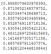
print('StratifiedKFold: Mean Accuracy Score = {}'.format(np.mean(scores)))
Apparently, the validation method used in connection with the data set used is not suitable. This could possibly be because the target values are very unbalanced. Let’s try another metric.
7.2.2 KFold
scores = cross_val_score(rf, trainX, trainY, cv=5)
scores
print('KFold: Mean Accuracy Score = {}'.format(np.mean(scores)))
That looks more realistic.
7.3 Hyperparameter optimization via Randomized Search
Let’s see how we can improve the model. We’ve usually done this with Grid Search so far. This time we use Randomized Search. This method is not so computationally intensive and therefore well suited for random forest.
rf_rand = RandomForestClassifier()param_dist = {"n_estimators": list(range(10,210,10)),
"max_depth": list(range(3,20)),
"max_features": list(range(1, 10)),
"min_samples_split": list(range(2, 11)),
"bootstrap": [True, False],
"criterion": ["gini", "entropy"]}n_iter_search = 50
random_search = RandomizedSearchCV(rf_rand, param_distributions=param_dist, scoring='accuracy',
n_iter=n_iter_search)
random_search.fit(trainX, trainY)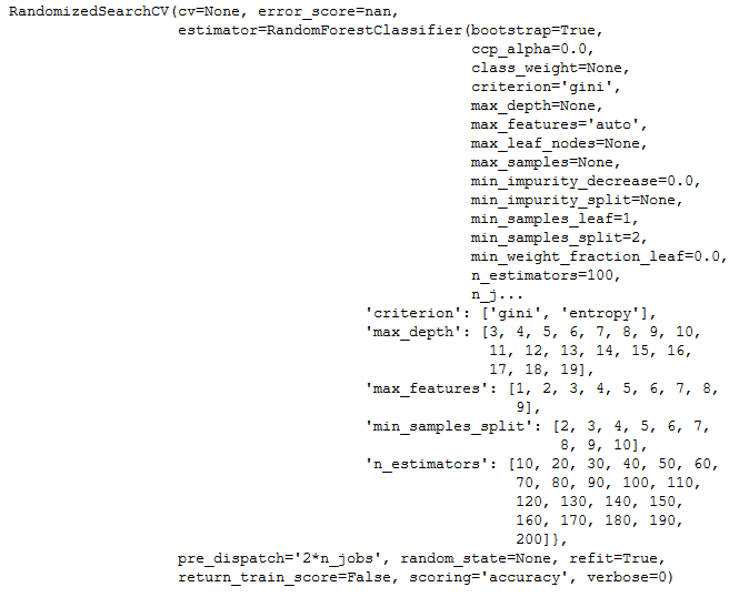
# View best hyperparameters
print('Best number of estimators:', random_search.best_estimator_.get_params()['n_estimators'])
print('Best min_samples_split:', random_search.best_estimator_.get_params()['max_depth'])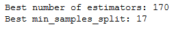
random_search.best_params_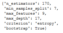
results = pd.DataFrame(random_search.cv_results_).sort_values('rank_test_score')
for i, row in results.head().iterrows():
    print("Model rank: {}".format(row.rank_test_score))
    print("Mean validation score: {:.3f} (std: {:.3f})".format(row.mean_test_score, row.std_test_score))
    print("Model Hyperparameters: {}\n".format(row.params))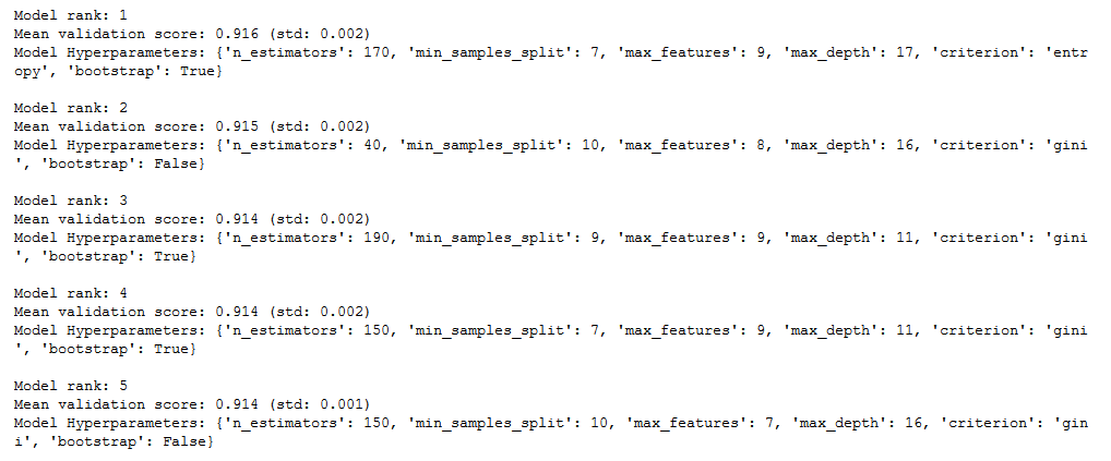
7.4 Determination of feature importance
feat_imps = pd.DataFrame({'importance': rf.feature_importances_}, index=bank.columns[:-1])
feat_imps.sort_values(by='importance', ascending=False, inplace=True)
feat_imps.plot(kind='bar', figsize=(10,7))
plt.legend()
plt.show()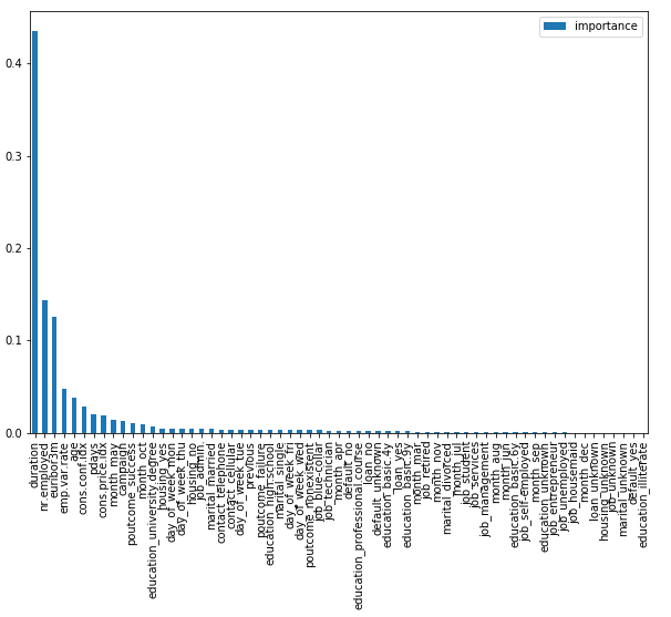
As we can see, very few features matter. It would therefore be worthwhile to use feature selection. How you can do this see here: “Feature selection methods for classification tasks”
8 Conclusion
In this post I showed what bagging is and how to use this ensemble method. Furthermore, I went into detail about the use of the Random Forest algorithm.
References
The content of the entire post was created using the following sources:
Johnston, B. & Mathur, I (2019). Applied Supervised Learning with Python. UK: Packt