1 Introduction
After “Bagging” and “Boosting” we come to the last type of ensemble method: Stacking.
For this post the dataset Bank Data from the platform “UCI Machine Learning Repository” was used. You can download it from my “GitHub Repository”.
2 Background Information on Stacking
The aim of this technique is to increase the predictie power of the classifier, as it involves training multiple models and then using a combiner algorithm to make the final prediction by using the predictions from all these models additional inputs.
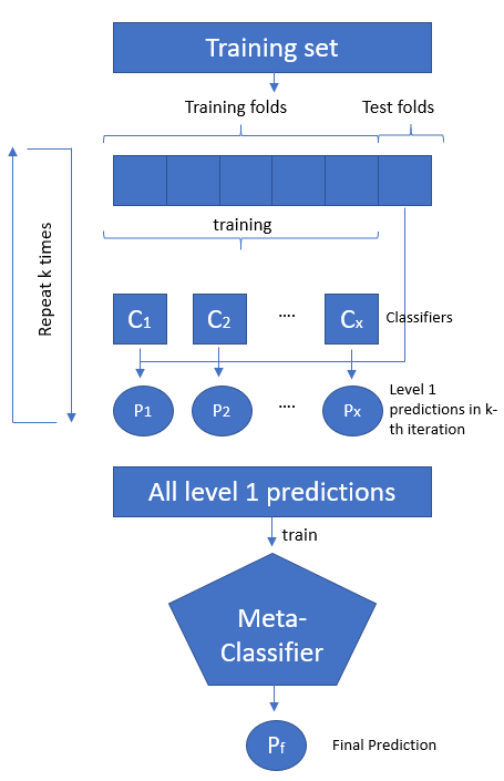
As you can see in the above pricture, this model ensembling technique combining information from multiple predictive models and using them as features to generate a new model. Stacking uses the predictions of the base models as additional features when training the final model… These are known as meta features. The stacked model essentially acts as a classifier that determines where each model is performing well and where it is performing poorly.
Let’s generate a stacked model step by step.
3 Loading the libraries and the data
import numpy as np
import pandas as pd
from sklearn.preprocessing import LabelBinarizer
from sklearn.model_selection import train_test_split


from sklearn.model_selection import KFold

# Our base models
from sklearn.neighbors import KNeighborsClassifier
from sklearn.svm import LinearSVC
# Our stacking model
from sklearn.linear_model import LogisticRegression

from sklearn.metrics import accuracy_score
bank = pd.read_csv("path/to/file/bank.csv", sep=";")
bank.head()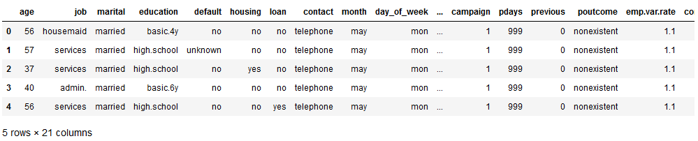
The data set before us contains information about whether a customer has signed a contract or not.
bank['y'].value_counts().T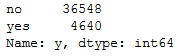
4 Data pre-processing
4.1 One-hot-encoding
First of all we have to convert the categorical variables into numerical ones again. To see how this work exactly please have a look at this post: “Types of Encoder”
safe_y = bank[['y']]

col_to_exclude = ['y']
bank = bank.drop(col_to_exclude, axis=1)
#Just select the categorical variables
cat_col = ['object']
cat_columns = list(bank.select_dtypes(include=cat_col).columns)
cat_data = bank[cat_columns]
cat_vars = cat_data.columns
#Create dummy variables for each cat. variable
for var in cat_vars:
cat_list = pd.get_dummies(bank[var], prefix=var)
bank=bank.join(cat_list)
data_vars=bank.columns.values.tolist()
to_keep=[i for i in data_vars if i not in cat_vars]
#Create final dataframe
bank_final=bank[to_keep]
bank_final.columns.values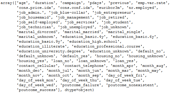
bank = pd.concat([bank_final, safe_y], axis=1)
bank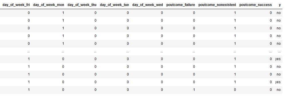
Now we have a data set that contains almost exclusively numerical variables. But as we can see, we still have to convert the target variable. We do not do this with one hot encoding but with the LabelBinarizer from scikit-learn.
4.2 LabelBinarizer
encoder = LabelBinarizer()

encoded_y = encoder.fit_transform(bank.y.values.reshape(-1,1))
encoded_y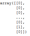
bank['y_encoded'] = encoded_y
bank['y_encoded'] = bank['y_encoded'].astype('int64')
bank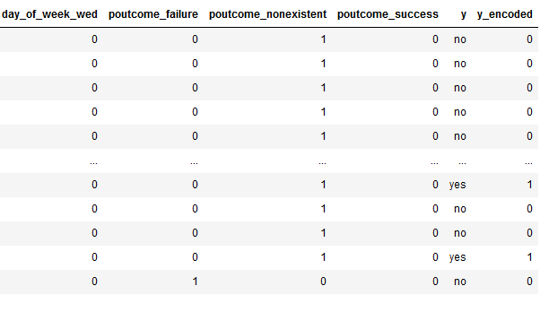
Here we see that the values of the newly generated target variables (here ‘y_encoded’) are now 0 or 1. Of course we can no longer take the ‘old’ target variable (here ‘y’) into account in the further evaluation. We will throw them out in the next step, the train-test-split.
4.3 Train-Test-Split
x = bank.drop(['y', 'y_encoded'], axis=1)
y = bank['y_encoded']

trainX, testX, trainY, testY = train_test_split(x, y, test_size = 0.2)
It is not a big deal.
4.4 Convert to a numpy array
For the following steps, it is necessary to convert the generated objects into numpy arrays.
trainX = trainX.to_numpy()
trainX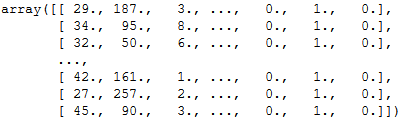
testX = testX.to_numpy()
testX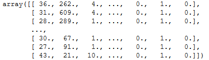
trainY = trainY.to_numpy()
trainY
testY = testY.to_numpy()
testY
5 Building a stacked model
In the following I will use a support vector machine (scikit-learns’s LinearSVC) and k-nearest neighbors (scikit-learn’s KneighboorsClassifier) as the base predictors and the stacked model will be a logistic regression classifier.
I explained the exact functioning of these algorithms in these posts:
5.1 Create a new training set
First of all we create a new training set with additional columns for predictions from base predictors.
trainX_with_metapreds = np.zeros((trainX.shape[0], trainX.shape[1]+2))
trainX_with_metapreds[:, :-2] = trainX
trainX_with_metapreds[:, -2:] = -1
print(trainX_with_metapreds)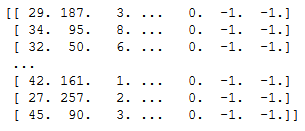
print(trainX.shape)
print(trainX_with_metapreds.shape)
Here we can see that two more columns have been added.
5.2 Train base models
Now we are going to train the base models using the k-fold strategy.
kf = KFold(n_splits=5, random_state=11)

for train_indices, test_indices in kf.split(trainX):
    kfold_trainX, kfold_testX = trainX[train_indices], trainX[test_indices]
    kfold_trainY, kfold_testY = trainY[train_indices], trainY[test_indices]

    svm = LinearSVC(random_state=11, max_iter=1000)
    svm.fit(kfold_trainX, kfold_trainY)
    svm_pred = svm.predict(kfold_testX)

    knn = KNeighborsClassifier(n_neighbors=4)
    knn.fit(kfold_trainX, kfold_trainY)
    knn_pred = knn.predict(kfold_testX)

    trainX_with_metapreds[test_indices, -2] = svm_pred
    trainX_with_metapreds[test_indices, -1] = knn_pred
5.3 Create a new test set
As I did in chapter 5.1, I will add two placeholder columns for the base model predictions in the test dataset as well.
testX_with_metapreds = np.zeros((testX.shape[0], testX.shape[1]+2))
testX_with_metapreds[:, :-2] = testX
testX_with_metapreds[:, -2:] = -1
print(testX_with_metapreds)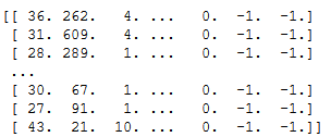
5.4 Fit base models on the complete training set
Next, I will train the two base predictors on the complete training set to get the meta prediction values for the test dataset. This is similar to what I did for each fold in chapter 5.2.
svm = LinearSVC(random_state=11, max_iter=1000)
svm.fit(trainX, trainY)

knn = KNeighborsClassifier(n_neighbors=4)
knn.fit(trainX, trainY)

svm_pred = svm.predict(testX)
knn_pred = knn.predict(testX)

testX_with_metapreds[:, -2] = svm_pred
testX_with_metapreds[:, -1] = knn_pred
5.5 Train the stacked model
The last step is to train the logistic regression model on all the columns of the training dataset plus the meta predictions rom the base estimators.
lr = LogisticRegression(random_state=11)
lr.fit(trainX_with_metapreds, trainY)
lr_preds_train = lr.predict(trainX_with_metapreds)
lr_preds_test = lr.predict(testX_with_metapreds)
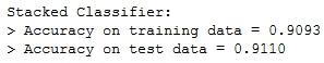
print('Stacked Classifier:\n> Accuracy on training data = {:.4f}\n> Accuracy on test data = {:.4f}'.format(
accuracy_score(y_true=trainY, y_pred=lr_preds_train),
accuracy_score(y_true=testY, y_pred=lr_preds_test)
))
6 Comparison of the accuracy
To get a sense of the performance boost from stacking, I will calculate the accuracies of the base predictors on the training and test dataset and compare it to that of the stacked model:
# Comparing accuracy with that of base predictors

print('SVM:\n> Accuracy on training data = {:.4f}\n> Accuracy on test data = {:.4f}'.format(
    accuracy_score(y_true=trainY, y_pred=svm.predict(trainX)),
    accuracy_score(y_true=testY, y_pred=svm_pred)
))
print('kNN:\n> Accuracy on training data = {:.4f}\n> Accuracy on test data = {:.4f}'.format(
    accuracy_score(y_true=trainY, y_pred=knn.predict(trainX)),
    accuracy_score(y_true=testY, y_pred=knn_pred)
))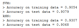
As we can see we get a higher accuracy on the test dataset with the stacked model as with the base predictors alone.
7 Conclusion
In this and in the last two posts I presented the use of various ensemble methods. It has been shown that the use of these methods leads to a significantly better result than the conventional machine learning algorithms alone.
References
The content of the entire post was created using the following sources:
Johnston, B. & Mathur, I (2019). Applied Supervised Learning with Python. UK: Packt