1 Introduction
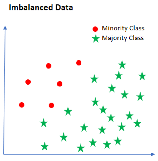
The validation metric ‚Accuracy‘ is a surprisingly common problem in machine learning (specifically in classification), occurring in datasets with a disproportionate ratio of observations in each class. Standard accuracy no longer reliably measures performance, which makes model training much trickier. Possibilities for dealing with imbalanced datasets should be dealt with in this publication.
For this post the dataset Bank Data from the platform “UCI Machine Learning repository” was used. You can download it from my “GitHub Repository”.
2 Loading the libraries and the data
import numpy as np
import pandas as pd

import seaborn as sns
import matplotlib.pyplot as plt

from sklearn.model_selection import train_test_split
from sklearn.metrics import accuracy_score
from sklearn.metrics import recall_score
from sklearn.metrics import roc_auc_score

#For chapter 4
from sklearn.linear_model import LogisticRegression

#For chapter 5
from sklearn.utils import resample

#For chapter 6.1
## You may need to install the following library:
## conda install -c glemaitre imbalanced-learn
from imblearn.over_sampling import SMOTE

#For chapter 6.2
from imblearn.under_sampling import NearMiss

#For chapter 7
from sklearn.svm import SVC

#For chapter 8
from sklearn.ensemble import RandomForestClassifier
bank = pd.read_csv("bank.csv", sep = ';')
bank = bank.rename(columns={'y':'final_subscribed'})Here we see that our target variable final_subscribed is distributed differently.
sns.countplot(x='final_subscribed', data=bank, palette='hls')
print(plt.show())
print(bank['final_subscribed'].value_counts())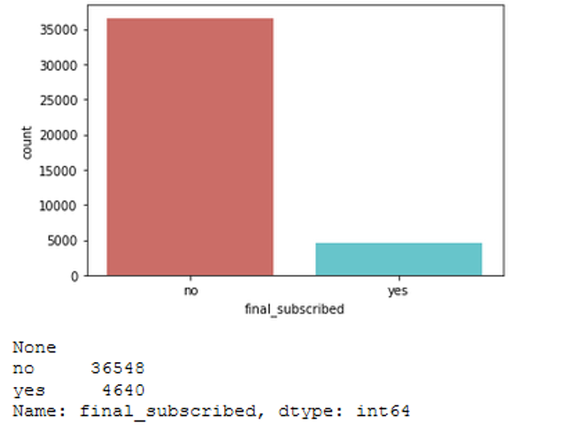
3 Data pre-processing
The use of this record requires some pre-processing steps (encoding of the target variable and one hot encoding of the categorial variables).
For a precise description of the data set and the pre-processing steps see my publication on “Logistic Regression”. I have already worked with the bank dataset here.
vals_to_replace = {'no':'0', 'yes':'1'}
bank['final_subscribed'] = bank['final_subscribed'].map(vals_to_replace)
bank['final_subscribed'] = bank.final_subscribed.astype('int64')
#Just select the categorical variables
cat_col = ['object']
cat_columns = list(bank.select_dtypes(include=cat_col).columns)
cat_data = bank[cat_columns]
cat_vars = cat_data.columns
#Create dummy variables for each cat. variable
for var in cat_vars:
cat_list = pd.get_dummies(bank[var], prefix=var)
bank=bank.join(cat_list)
data_vars=bank.columns.values.tolist()
to_keep=[i for i in data_vars if i not in cat_vars]
#Create final dataframe
bank_final=bank[to_keep]The final data record we received now has 41,188 rows and 64 columns.
bank_final.shape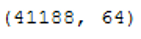
4 Logistic Regression
Predicting whether a customer will finally subscribed is a classic binary classification problem. We can use logistic regression for this.
x = bank_final.drop('final_subscribed', axis=1)
y = bank_final['final_subscribed']

trainX, testX, trainY, testY = train_test_split(x, y, test_size = 0.2)
clf_0_LogReg = LogisticRegression()
clf_0_LogReg.fit(trainX, trainY)
y_pred = clf_0_LogReg.predict(testX)
print('Accuracy: {:.2f}'.format(accuracy_score(testY, y_pred)))
Accuracy of 0.91 not bad ! But what about recall? If you are not familiar with this metric look at this “Post (Chapter 6.3.2 Further metrics)”.
recall_score(testY, y_pred)
Mh ok … 0.38 is not the best value. Maybe this is because the target class is imbalanced?
Let’s see how we can fix this problem and what the other models deliver for results. The RocAuc-Score is a good way to compare the models with one another.
prob_y_0 = clf_0_LogReg.predict_proba(testX)[::,1]

roc_auc_score(testY, prob_y_0)
5 Resampling methods
A widely adopted technique for dealing with highly unbalanced dataframes is called resampling. It consists of removing samples from the majority class (under-sampling) and/or adding more examples from the minority class (over-sampling). Despite the advantage of balancing classes, these techniques also have their weaknesses. You know there is no free lunch.
The simplest implementation of over-sampling is to duplicate random records from the minority class, which can cause overfitting. In under-sampling, the simplest technique involves removing random records from the majority class, which can cause loss of information. I will show both methods below.
5.1 Oversampling
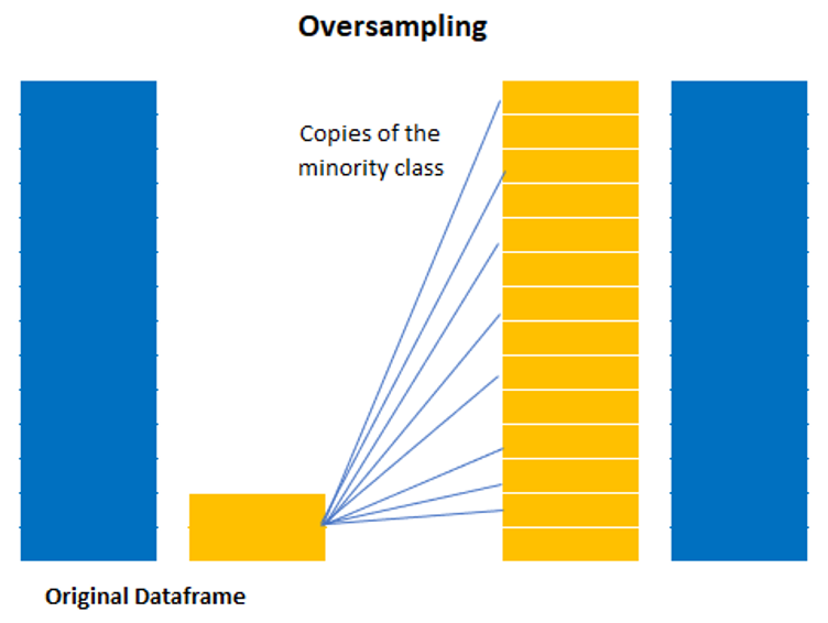
Oversampling or up-sampling is the process of randomly duplicating observations from the minority class in order to reinforce its signal.
There are several heuristics for doing so, but the most common way is to simply resample with replacement:
- First, we’ll separate observations from each class into different datasets.
- Next, we’ll resample the minority class with replacement, setting the number of samples to match that of the majority class.
- Finally, we’ll combine the up-sampled minority class dataset with the original majority class dataset.
First let’s take a quick look at the exact distribution of the target variable.
print(bank_final['final_subscribed'].value_counts())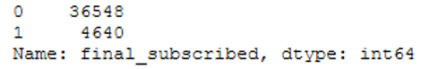
# Separate majority and minority classes
df_majority = bank_final[bank_final.final_subscribed==0]
df_minority = bank_final[bank_final.final_subscribed==1]

# Upsample minority class
df_minority_upsampled = resample(df_minority,
                                 replace=True,      # sample with replacement
                                 n_samples=36548)   # to match majority class


#Combine majority class with upsampled minority class
df_upsampled = pd.concat([df_majority, df_minority_upsampled])
Below we see that our data set is now balanced.
print(df_upsampled['final_subscribed'].value_counts())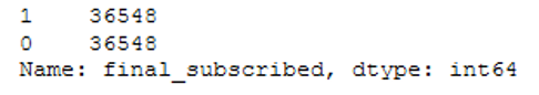
Let’s train the Logisitc Regression model again.
x = df_upsampled.drop('final_subscribed', axis=1)
y = df_upsampled['final_subscribed']

trainX, testX, trainY, testY = train_test_split(x, y, test_size = 0.2)
clf_1_LogReg = LogisticRegression()
clf_1_LogReg.fit(trainX, trainY)
y_pred = clf_1_LogReg.predict(testX)
print('Accuracy: {:.2f}'.format(accuracy_score(testY, y_pred)))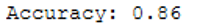
We see that the accuracy has decreased. What about recall?
recall_score(testY, y_pred)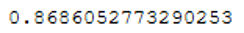
Looks better! For a later model comparison we calculate the RocAuc-Score.
prob_y_1 = clf_1_LogReg.predict_proba(testX)[::,1]

roc_auc_score(testY, prob_y_1)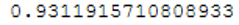
5.2 Undersampling
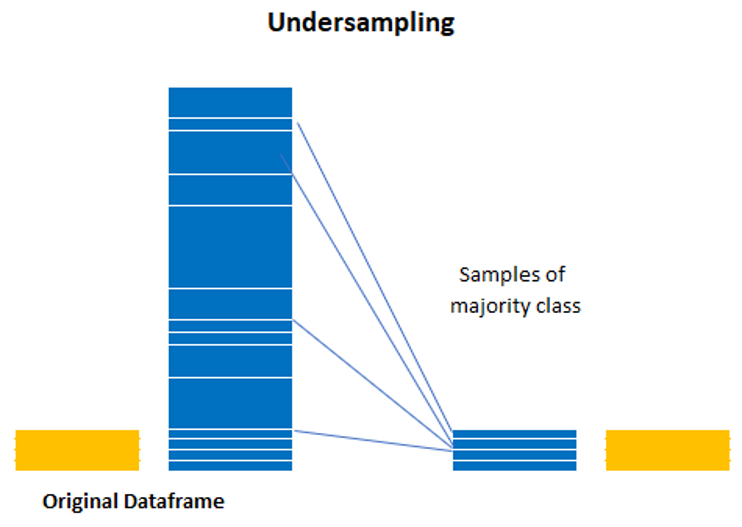
Undersampling or down-sampling involves randomly removing observations from the majority class to prevent its signal from dominating the learning algorithm. The most common heuristic for doing so is resampling without replacement.
The process is quite similar to that of up-sampling. Here are the steps:
- First, we’ll separate observations from each class into different datasets.
- Next, we’ll resample the majority class without replacement, setting the number of samples to match that of the minority class.
- Finally, we’ll combine the down-sampled majority class dataset with the original minority class dataset.
# Separate majority and minority classes
df_majority = bank_final[bank_final.final_subscribed==0]
df_minority = bank_final[bank_final.final_subscribed==1]

# Downsample majority class
df_majority_downsampled = resample(df_majority,
                                 replace=False,     # sample without replacement
                                 n_samples=4640)    # to match minority class

# Combine minority class with downsampled majority class
df_downsampled = pd.concat([df_majority_downsampled, df_minority])
We see a balanced record again.
print(df_downsampled['final_subscribed'].value_counts())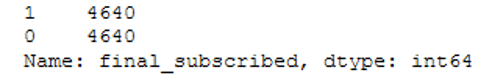
Let’s train a further Logisitc Regression model and have a look at the metrics.
x = df_downsampled.drop('final_subscribed', axis=1)
y = df_downsampled['final_subscribed']

trainX, testX, trainY, testY = train_test_split(x, y, test_size = 0.2)
clf_2_LogReg = LogisticRegression()
clf_2_LogReg.fit(trainX, trainY)
y_pred = clf_2_LogReg.predict(testX)
print('Accuracy: {:.2f}'.format(accuracy_score(testY, y_pred)))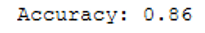
recall_score(testY, y_pred)
prob_y_2 = clf_2_LogReg.predict_proba(testX)[::,1]

roc_auc_score(testY, prob_y_2)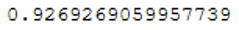
6 ML Algorithms for imbalanced datasets
Following we’ll discuss two of the common and simple ways to deal with the problem of unbalanced classes using machine learning algorithms.
6.1 SMOTE (Synthetic Minority Over-sampling Technique)
SMOTE is an over-sampling method. What it does is, it creates synthetic (not duplicate) samples of the minority class. Hence making the minority class equal to the majority class. SMOTE does this by selecting similar records and altering that record one column at a time by a random amount within the difference to the neighbouring records.
x = bank_final.drop('final_subscribed', axis=1)
y = bank_final['final_subscribed']

trainX, testX, trainY, testY = train_test_split(x, y, test_size = 0.2)
columns_x = trainX.columns
sm = SMOTE()
trainX_smote ,trainY_smote = sm.fit_resample(trainX, trainY)
trainX_smote = pd.DataFrame(data=trainX_smote,columns=columns_x)
trainY_smote = pd.DataFrame(data=trainY_smote,columns=['final_subscribed'])print("Before OverSampling, counts of label '1': {}".format(sum(trainY==1)))
print("Before OverSampling, counts of label '0': {} \n".format(sum(trainY==0)))
print("After OverSampling, counts of label '1':", trainY_smote[(trainY_smote["final_subscribed"] == 1)].shape[0])
print("After OverSampling, counts of label '0':", trainY_smote[(trainY_smote["final_subscribed"] == 0)].shape[0])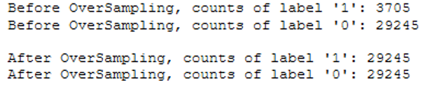
clf_3_LogReg = LogisticRegression()
clf_3_LogReg.fit(trainX_smote, trainY_smote)

y_pred = clf_3_LogReg.predict(testX)

print('Accuracy: {:.2f}'.format(accuracy_score(testY, y_pred)))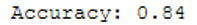
recall_score(testY, y_pred)
prob_y_3 = clf_3_LogReg.predict_proba(testX)[::,1]

roc_auc_score(testY, prob_y_3)
6.2 NearMiss
NearMiss is an under-sampling technique. Instead of resampling the Minority class, using a distance, this will make the majority class equal to minority class.
x = bank_final.drop('final_subscribed', axis=1)
y = bank_final['final_subscribed']

trainX, testX, trainY, testY = train_test_split(x, y, test_size = 0.2)
columns_x = trainX.columns
NearM = NearMiss()
trainX_NearMiss ,trainY_NearMiss = NearM.fit_resample(trainX, trainY)
trainX_NearMiss = pd.DataFrame(data=trainX_NearMiss,columns=columns_x)
trainY_NearMiss = pd.DataFrame(data=trainY_NearMiss,columns=['final_subscribed'])print("Before UnderSampling, counts of label '1': {}".format(sum(trainY==1)))
print("Before UnderSampling, counts of label '0': {} \n".format(sum(trainY==0)))
print("After UnderSampling, counts of label '1':", trainY_NearMiss[(trainY_NearMiss["final_subscribed"] == 1)].shape[0])
print("After UnderSampling, counts of label '0':", trainY_NearMiss[(trainY_NearMiss["final_subscribed"] == 0)].shape[0])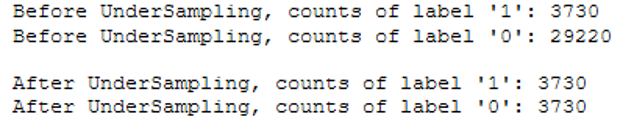
clf_4_LogReg = LogisticRegression()
clf_4_LogReg.fit(trainX_NearMiss, trainY_NearMiss)

y_pred = clf_4_LogReg.predict(testX)

print('Accuracy: {:.2f}'.format(accuracy_score(testY, y_pred)))
recall_score(testY, y_pred)
prob_y_4 = clf_4_LogReg.predict_proba(testX)[::,1]

roc_auc_score(testY, prob_y_4)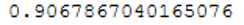
7 Penalize Algorithms
The next possibility is to use penalized learning algorithms that increase the cost of classification mistakes on the minority class. A popular algorithm for this technique is Penalized-SVM:
x = bank_final.drop('final_subscribed', axis=1)
y = bank_final['final_subscribed']

trainX, testX, trainY, testY = train_test_split(x, y, test_size = 0.2)
clf_SVC = SVC(kernel='linear',
class_weight='balanced', # penalize
probability=True)
clf_SVC.fit(trainX, trainY)
y_pred = clf_SVC.predict(testX)
print('Accuracy: {:.2f}'.format(accuracy_score(testY, y_pred)))
recall_score(testY, y_pred)
prob_y_SVM = clf_SVC.predict_proba(testX)[::,1]

roc_auc_score(testY, prob_y_SVM)
8 Tree-Based Algorithms
The final possibility we’ll consider is using tree-based algorithms. Decision trees often perform well on imbalanced datasets because their hierarchical structure allows them to learn signals from both classes.
x = bank_final.drop('final_subscribed', axis=1)
y = bank_final['final_subscribed']

trainX, testX, trainY, testY = train_test_split(x, y, test_size = 0.2)
clf_RFC = RandomForestClassifier()
clf_RFC.fit(trainX, trainY)
y_pred = clf_RFC.predict(testX)
print('Accuracy: {:.2f}'.format(accuracy_score(testY, y_pred)))
recall_score(testY, y_pred)
prob_y_RFC = clf_RFC.predict_proba(testX)[::,1]

roc_auc_score(testY, prob_y_RFC)
9 Conclusion
In this post I showed what effects imbalanced dataframes can have on the creation of machine learning models, which metrics can be used to measure actual performance and what can be done with imbalanced dataframes in order to be able to train machine learning models with them.
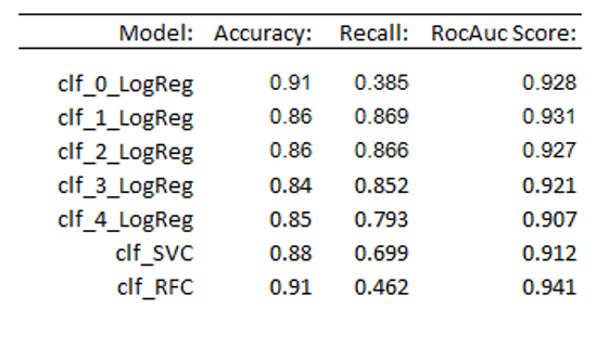
Here is an overview of the metrics of the models used in this publication: