1 Introduction
In my last post about Deep Learning with the Multi-layer Perceptron, I showed how to make classifications with this type of neural network.
However, an MLP can also be used to solve regression problems. This will be the content of the following post.
For this publication the dataset House Sales in King County, USA from the statistic platform “Kaggle” was used. You can download it from my “GitHub Repository”.
2 Loading the libraries and data
import pandas as pd
import numpy as np

import matplotlib.pyplot as plt

from sklearn.model_selection import train_test_split
from sklearn.preprocessing import StandardScaler

from sklearn.neural_network import MLPRegressor

from sklearn import metrics

from sklearn.model_selection import GridSearchCV
df = pd.read_csv('house_prices.csv')
df = df.drop(['id', 'date', 'yr_built', 'yr_renovated', 'zipcode', 'lat', 'long'], axis=1)
df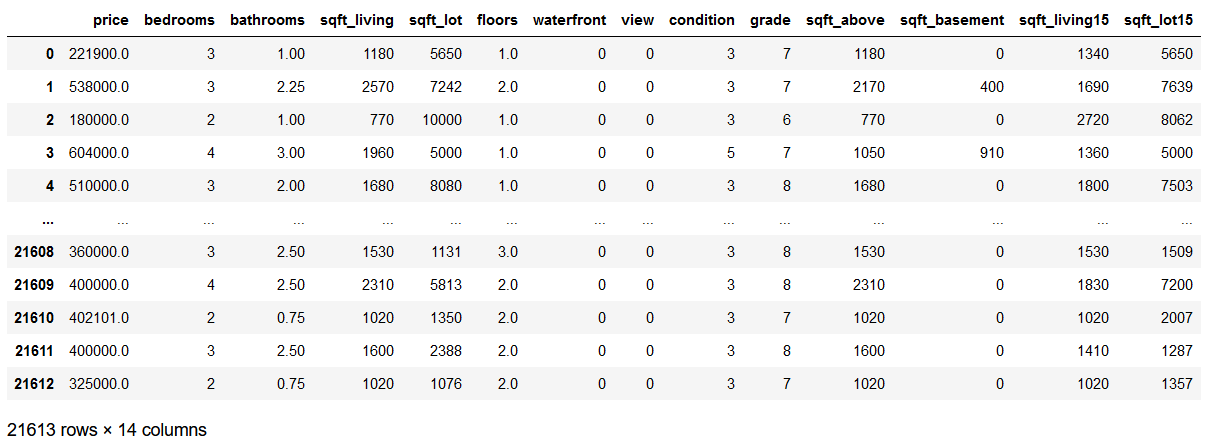
3 Data pre-processing
x = df.drop('price', axis=1)
y = df['price']

trainX, testX, trainY, testY = train_test_split(x, y, test_size = 0.2)
sc=StandardScaler()
scaler = sc.fit(trainX)
trainX_scaled = scaler.transform(trainX)
testX_scaled = scaler.transform(testX)4 MLPRegressor
mlp_reg = MLPRegressor(hidden_layer_sizes=(150,100,50),
                       max_iter = 300,activation = 'relu',
                       solver = 'adam')

mlp_reg.fit(trainX_scaled, trainY)
5 Model Evaluation
y_pred = mlp_reg.predict(testX_scaled)df_temp = pd.DataFrame({'Actual': testY, 'Predicted': y_pred})
df_temp.head()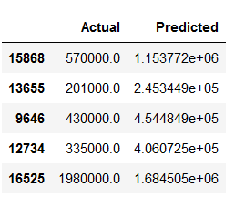
df_temp = df_temp.head(30)
df_temp.plot(kind='bar',figsize=(10,6))
plt.grid(which='major', linestyle='-', linewidth='0.5', color='green')
plt.grid(which='minor', linestyle=':', linewidth='0.5', color='black')
plt.show()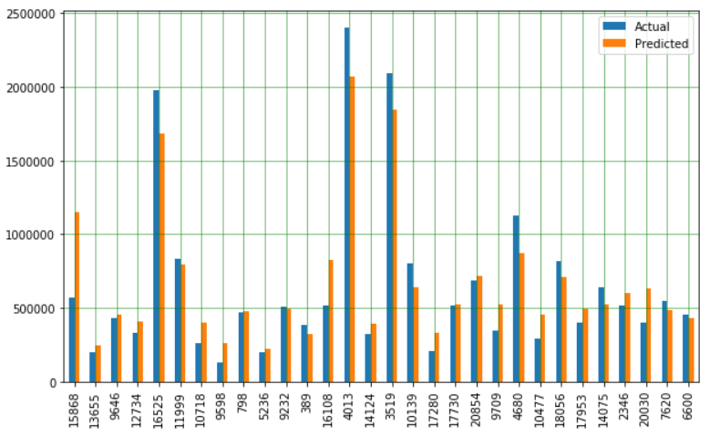
print('Mean Absolute Error:', metrics.mean_absolute_error(testY, y_pred))
print('Mean Squared Error:', metrics.mean_squared_error(testY, y_pred))
print('Root Mean Squared Error:', np.sqrt(metrics.mean_squared_error(testY, y_pred)))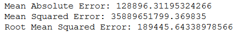
What these metrics mean and how to interpret them I have described in the following post: Metrics for Regression Analysis
plt.plot(mlp_reg.loss_curve_)
plt.title("Loss Curve", fontsize=14)
plt.xlabel('Iterations')
plt.ylabel('Cost')
plt.show()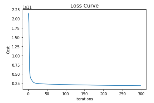
6 Hyper Parameter Tuning
param_grid = {
    'hidden_layer_sizes': [(150,100,50), (120,80,40), (100,50,30)],
    'max_iter': [50, 100],
    'activation': ['tanh', 'relu'],
    'solver': ['sgd', 'adam'],
    'alpha': [0.0001, 0.05],
    'learning_rate': ['constant','adaptive'],
}
grid = GridSearchCV(mlp_reg, param_grid, n_jobs= -1, cv=5)
grid.fit(trainX_scaled, trainY)
print(grid.best_params_) 
grid_predictions = grid.predict(testX_scaled) df_temp2 = pd.DataFrame({'Actual': testY, 'Predicted': grid_predictions})
df_temp2.head()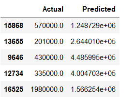
df_temp2 = df_temp2.head(30)
df_temp2.plot(kind='bar',figsize=(10,6))
plt.grid(which='major', linestyle='-', linewidth='0.5', color='green')
plt.grid(which='minor', linestyle=':', linewidth='0.5', color='black')
plt.show()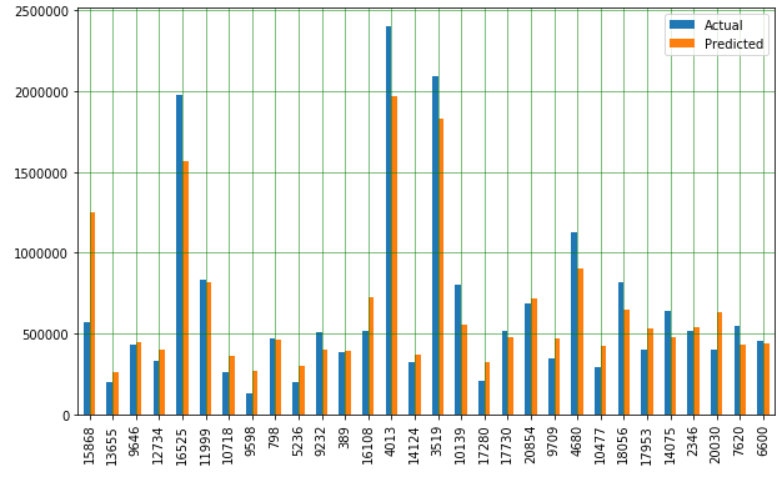
print('Mean Absolute Error:', metrics.mean_absolute_error(testY, grid_predictions))
print('Mean Squared Error:', metrics.mean_squared_error(testY, grid_predictions))
print('Root Mean Squared Error:', np.sqrt(metrics.mean_squared_error(testY, grid_predictions)))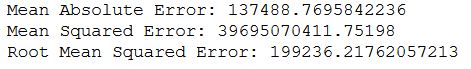
What these metrics mean and how to interpret them I have described in the following post: Metrics for Regression Analysis
7 Conclusion
In this post, I showed how to solve regression problems using the MLPRegressor. In subsequent posts, I will show how to perform classifications and regressions using the deep learning library Keras.