1 Introduction
In addition to “Logistic Regression”, there is another very well-known algorithm for binary classifications: the Support Vector Machine (SVM).
For this post the dataset Breast Cancer Wisconsin (Diagnostic) from the statistic platform “Kaggle” was used. You can download it from my GitHub Repository.
2 Background information on Support Vector Machines
What is Support Vector Machine?
“Support Vector Machine” (SVM) is a supervised machine learning algorithm which can be used for both classification or regression problems.
However, SVM is mostly used in classification problems.
Like logistic regression, SVM is one of the binary classification algorithms. However, both LogReg and SVM can also be used for multiple classification problems. This will be dealt with in a separate post.
The core idea of SVM is to find a maximum marginal hyperplane (MMH) that best divides the dataset into classes (see picture below).
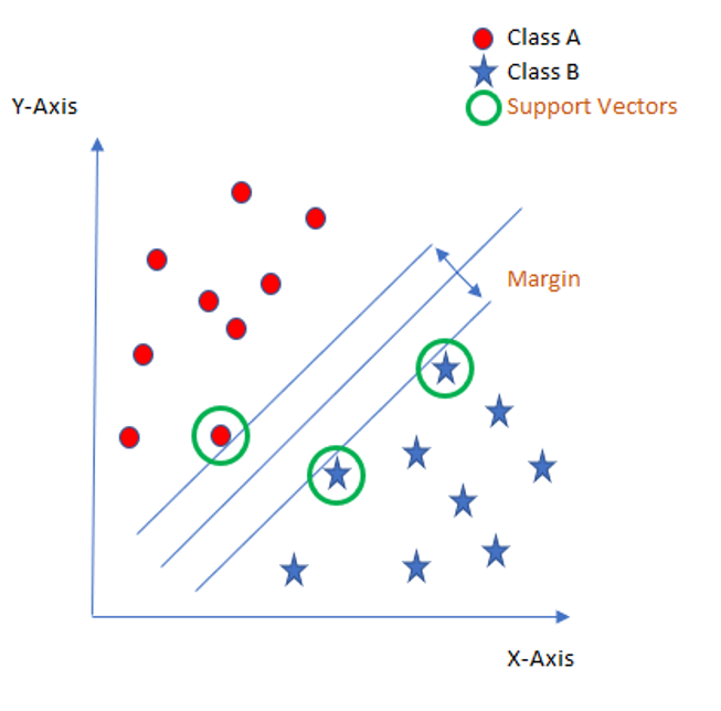
Support Vectors
The support vectors are the data points, which are closest to the so called hyperplane. These points will define the separating line better by calculating margins.
Hyperplane
A hyperplane is a decision plane which separates between a set of objects having different class memberships.
Margin
The margin is the gap between the two lines on the closest class points. This is calculated as the perpendicular distance from the line to support vectors or closest points. If the margin is larger in between the classes, then it is considered a good margin, a smaller margin is a bad margin.
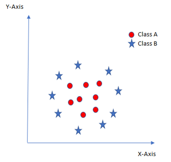
Some problems can’t be solved using linear hyperplane, as shown in the following figure:
In such situation, SVM uses a kernel trick to transform the input space to a higher dimensional space as shown here:
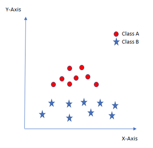
Now the two classes can be easily separated from each other again.
Jiapu Zhang provides “here” a complete list of kernels used in SVMs.
There are several pos and cons for the use of Support Vector Machines:
Pros:
- SVM works relatively well when there is clear margin of separation between classes.
- Effective in high dimensional spaces.
- Still effective in cases where number of dimensions is greater than the number of samples.
- Uses a subset of training points in the decision function (called support vectors), so it is also memory efficient.
- Versatile: different Kernel functions can be specified for the decision function. Common kernels are provided, but it is also possible to specify custom kernels.
Cons:
- SVM algorithm is not suitable for large data sets.
- SVM does not perform very well, when the data set has more noise i.e. target classes are overlapping.
- If the number of features is much greater than the number of samples, avoid over-fitting in choosing Kernel functions and regularization term is crucial.
- SVMs do not directly provide probability estimates, these are calculated using an expensive five-fold cross-validation.
3 Loading the libraries and the data
import pandas as pd
import numpy as np

# for chapter 5.1
from sklearn.model_selection import train_test_split
from sklearn.svm import SVC

# for chapter 5.2
from sklearn.metrics import confusion_matrix
from sklearn.metrics import accuracy_score
from sklearn.metrics import precision_score
from sklearn.metrics import recall_score
from sklearn.metrics import f1_score
from sklearn.model_selection import cross_val_score
# for chapter 7
from sklearn.model_selection import GridSearchCV
cancer = pd.read_csv("path/to/file/breast_cancer.csv")cancer.head()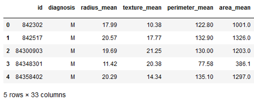
The data set used contains 31 columns which contain information about tumors in the tissue. The column ‘diagnosis’ describes whether these tumors are benign (B) or malignant (M). Let’s try to create a classification model.
4 Data pre-processing
The target variable is then converted into numerical values.
vals_to_replace = {'B':'0', 'M':'1'}
cancer['diagnosis'] = cancer['diagnosis'].map(vals_to_replace)
cancer['diagnosis'] = cancer.diagnosis.astype('int64')
cancer.head()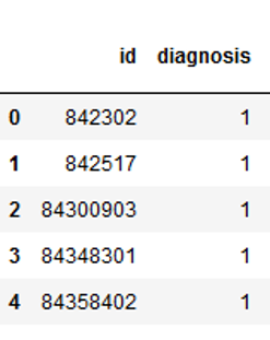
5 SVM with scikit-learn
5.1 Model Fitting
In the case of a simple Support Vector Machine we simply set this parameter as “linear” since simple SVMs can only classify linearly separable data. We will see non-linear kernels in chapter 6.
The variables ‘id’ and ‘Unnamed: 32’ are excluded because the ID is not profitable and Unnamed: 32 only contains missing values.
x = cancer.drop(['id', 'diagnosis', 'Unnamed: 32'], axis=1)
y = cancer['diagnosis']

trainX, testX, trainY, testY = train_test_split(x, y, test_size = 0.2)

clf = SVC(kernel='linear')
clf.fit(trainX, trainY)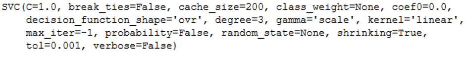
y_pred = clf.predict(testX)5.2 Model evaluation
For the model evaluation we start again with the confusion matrix
confusion_matrix = confusion_matrix(testY, y_pred)
print(confusion_matrix)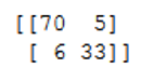
Some more metrics follow:
print('Accuracy: {:.2f}'.format(accuracy_score(testY, y_pred)))
print('Error rate: {:.2f}'.format(1 - accuracy_score(testY, y_pred)))
print('Precision: {:.2f}'.format(precision_score(testY, y_pred)))
print('Recall: {:.2f}'.format(recall_score(testY, y_pred)))
print('f1_score: {:.2f}'.format(f1_score(testY, y_pred)))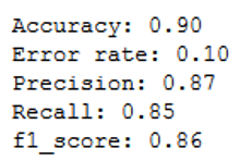
Okay, let’s see what the cross validation results for.
clf = SVC(kernel='linear')
scores = cross_val_score(clf, trainX, trainY, cv=5)
scores
print("Accuracy: %0.2f (+/- %0.2f)" % (scores.mean(), scores.std() * 2))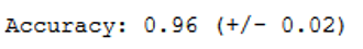
Using cross validation, we achieved an accuracy rate of 0.96. Previously it was only 0.90. Before we get into hyper-parameter optimization, let’s see if using a different kernel can improve the accuracy of the classification.
6 Kernel SVM with Scikit-Learn
6.1 Polynomial Kernel
In the case of polynomial kernel, you also have to pass a value for the degree parameter of the SVM class. This basically is the degree of the polynomial. Take a look at how we can use a polynomial kernel to implement kernel SVM. Finally, the accuracy rate is calculated again.
clf_poly = SVC(kernel='poly', degree=8)
clf_poly.fit(trainX, trainY)
y_pred = clf_poly.predict(testX)
print('Accuracy: {:.2f}'.format(accuracy_score(testY, y_pred)))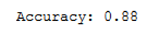
At 0.88 we are slightly worse than with the linear kernel.
6.2 Gaussian Kernel
If the gaussian kernel is to be used, “rbf” must be entered as kernel:
clf_rbf = SVC(kernel='rbf')
clf_rbf.fit(trainX, trainY)
y_pred = clf_rbf.predict(testX)
print('Accuracy: {:.2f}'.format(accuracy_score(testY, y_pred)))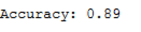
Here the accuracy rate is slightly higher but still lower than of the linear kernel
6.3 Sigmoid Kernel
If the sigmoid kernel is to be used, “sigmoid” must be entered as kernel:
clf_sigmoid = SVC(kernel='sigmoid')
clf_sigmoid.fit(trainX, trainY)
y_pred = clf_sigmoid.predict(testX)
print('Accuracy: {:.2f}'.format(accuracy_score(testY, y_pred)))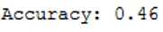
The accuracy rate is very bad.
7 Hyperparameter optimization via Grid Search
Since the use of the linear kernel has yielded the best results so far, an attempt is made to optimize the hypter parameters in this kernel.
param_grid = {'C': [0.1, 1, 10, 100, 1000],
              'gamma': [1, 0.1, 0.01, 0.001, 0.0001],
              'kernel': ['linear']}
grid = GridSearchCV(SVC(), param_grid, cv = 5, scoring='accuracy')
grid.fit(trainX, trainY) 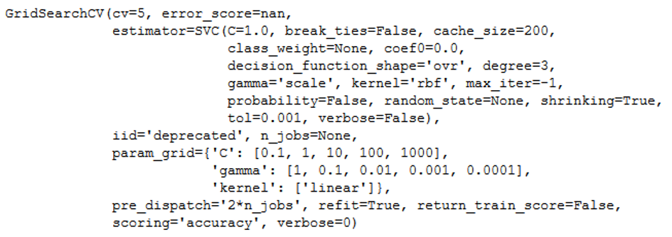
With best_params_ we get the best fitting values:
print(grid.best_params_) 
print(grid.best_estimator_) 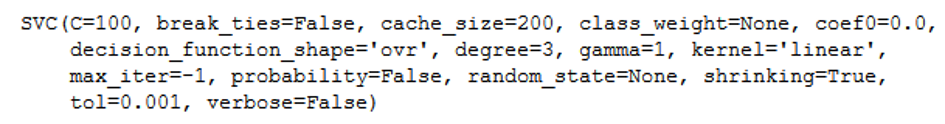
We can also use the model trained with GridSearch (here “grid”) to predict the test data set:
grid_predictions = grid.predict(testX) Now let’s see if the optimization has achieved anything:
print('Accuracy: {:.2f}'.format(accuracy_score(testY, grid_predictions)))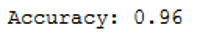
Yeah, accuracy of 0.96 !
With GridSearch we can also compare all available kernels with corresponding hyper parameters. Use this syntax to do so:
param_grid_full = [
  {'kernel': ['linear'], 'C': [0.001, 0.10, 0.1, 10, 25, 50, 100, 1000]},
  {'kernel': ['rbf'], 'C': [0.001, 0.10, 0.1, 10, 25, 50, 100, 1000],
    'gamma': [1, 0.1, 0.01, 0.001, 0.0001, 0.00001]},
  {'kernel': ['sigmoid'], 'C': [0.001, 0.10, 0.1, 10, 25, 50, 100, 1000],
    'gamma': [1, 0.1, 0.01, 0.001, 0.0001, 0.00001]},
 ]

grid_full = GridSearchCV(SVC(), param_grid_full, cv = 10, scoring='accuracy')
grid_full.fit(trainX, trainY) 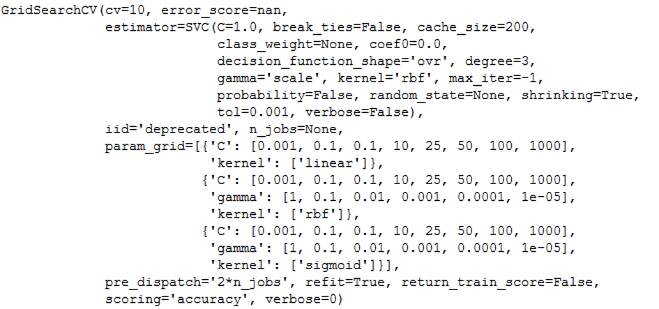
print(grid_full.best_params_) 
grid_predictions = grid_full.predict(testX)

print('Accuracy: {:.2f}'.format(accuracy_score(testY, grid_predictions)))
Although we could not further increase the accuracy with the large grid search procedure. The output of the best parameters shows that the kernel ‘rbf’ with the corresponding C and gamma is the model of choice. It should be noted that this is very computationally intensive.
8 Conclusion
This post showed how to use Support Vector Machines with different kernels and how to measure their performance. Furthermore, the improvement of the models was discussed.