1 Introduction
My previous posts were mostly about treating regression problems. Now we’ll change from regression to classification. Let’s start with the introduction of a binary classification algorithm: Logistic Regression
For this post the dataset Bank Data from the platform “UCI Machine Learning repository” was used. You can download it from my GitHub Repository.
2 Loading the libraries and the data
import numpy as np
import pandas as pd

import statsmodels.api as sm
import seaborn as sns
import matplotlib.pyplot as plt
%matplotlib inline
sns.set(style="white")
sns.set(style="whitegrid", color_codes=True)


from sklearn.model_selection import train_test_split


#for chapter 4.3
from sklearn.feature_selection import RFE

#for chapter 4.3 and 6.2
from sklearn.linear_model import LogisticRegression

#for chapter 5
import statsmodels.api as sm

#for chapter 6.1
## You may need to install the following library:
## conda install -c glemaitre imbalanced-learn
from imblearn.over_sampling import SMOTE

#for chapter 6.3
from sklearn.metrics import accuracy_score
from sklearn.metrics import precision_score
from sklearn.metrics import recall_score
from sklearn.metrics import f1_score

from sklearn.metrics import confusion_matrix

from sklearn.metrics import roc_auc_score
from sklearn.metrics import roc_curve
from sklearn.tree import DecisionTreeClassifier
from sklearn.ensemble import RandomForestClassifier
from sklearn.metrics import plot_roc_curve


from sklearn.model_selection import cross_val_score
bank = pd.read_csv("bank.csv", sep = ';')
bank = bank.rename(columns={'y':'final_subscribed'})
bank.head().T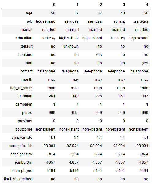
Here we have a small overview of the variables from the data set to be analyzed. A detailed description of the variables is given at the end of this publication. Our target variable is final_subscribed which means whether a customer has finally signed or not.
3 Descriptive statistics
3.1 Mean values of the features
#Overview of the mean values of the features grouped by final_subscribed
df = bank.groupby('final_subscribed').mean().T

#Compilation of the difference between the mean values
col_names = df.columns
df = pd.DataFrame(df, columns = col_names)
df['Score_diff'] = df['no'] - df['yes']
df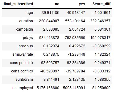
#Filter for differences below -2 and above 2
threshold = ['2', '-2']
df[(df["Score_diff"] >= float(threshold[0])) | (df["Score_diff"] <= float(threshold[1]))]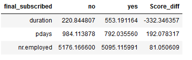
3.2 Description of the target variable
sns.countplot(x='final_subscribed', data=bank, palette='hls')
print(plt.show())
print(bank['final_subscribed'].value_counts())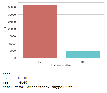
#get percentage of male and female within our dataset

bank['final_subscribed'].value_counts(normalize=True) * 100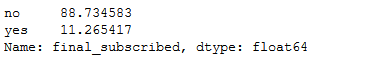
3.3 Description of the predictor variables
%matplotlib inline
pd.crosstab(bank.job, bank.final_subscribed).plot(kind='bar')
plt.title('Subscription Frequency for Job Title')
plt.xlabel('Job')
plt.ylabel('Frequency of subscriptions')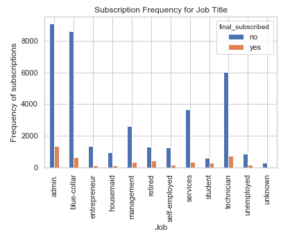
The job title can be a good predictor for final subscription.
%matplotlib inline
pd.crosstab(bank.day_of_week, bank.final_subscribed).plot(kind='bar')
plt.title('Subscription Frequency for Day of Week')
plt.xlabel('Day of Week')
plt.ylabel('Frequency of subscriptions')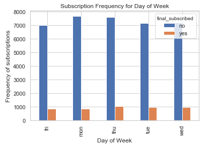
Day of week may not be a good predictor of for final subscription.
%matplotlib inline
pd.crosstab(bank.month, bank.final_subscribed).plot(kind='bar')
plt.title('Subscription Frequency for Month')
plt.xlabel('Month')
plt.ylabel('Frequency of subscriptions')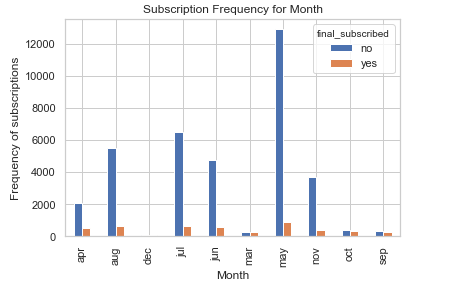
The month can be a good predictor for final subscription.
%matplotlib inline
pd.crosstab(bank.education, bank.final_subscribed).plot(kind='bar')
plt.title('Subscription Frequency for Education')
plt.xlabel('Education')
plt.ylabel('Frequency of subscriptions')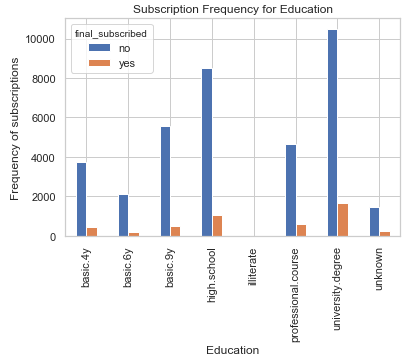
The Education can be a good predictor for final subscription.
bank.age.hist()
plt.title('Histogram of Age')
plt.xlabel('Age')
plt.ylabel('Frequency')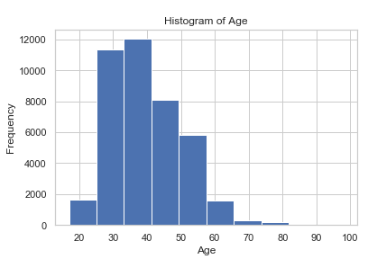
On the more detailed examination of the remaining variables is omitted in this post.
4 Data pre-processing
4.1 Conversion of the target variable
vals_to_replace = {'no':'0', 'yes':'1'}
bank['final_subscribed'] = bank['final_subscribed'].map(vals_to_replace)
bank['final_subscribed'] = bank.final_subscribed.astype('int64')
bank.head()
Now we have 0 and 1 as int64 for our target variable
4.2 Creation of dummy variables
There are some categorical variables in the data set. A logistic regression model only works with numeric variables, so we have to convert the non-numeric ones to dummy variables. If you want to learn more about one-hot-encoding / dummy variables, read this post from me: “The use of dummy variables”
#Just select the categorical variables
cat_col = ['object']
cat_columns = list(bank.select_dtypes(include=cat_col).columns)
cat_data = bank[cat_columns]
cat_vars = cat_data.columns

#Create dummy variables for each cat. variable
for var in cat_vars:
    cat_list = pd.get_dummies(bank[var], prefix=var)
    bank=bank.join(cat_list)


data_vars=bank.columns.values.tolist()
to_keep=[i for i in data_vars if i not in cat_vars]

#Create final dataframe
bank_final=bank[to_keep]
bank_final.columns.values
4.3 Feature Selection
Now we have created some new variables. However, not all are relevant for the planned classification. We use the Recursive Feature Elimination (RFE) algorithm to eliminate the redundant features.
#Here we select 20 best features

x = bank_final.drop('final_subscribed', axis=1)
y = bank_final['final_subscribed']

trainX, testX, trainY, testY = train_test_split(x, y, test_size = 0.2)

model = LogisticRegression()
rfe = RFE(model, 20)
fit = rfe.fit(trainX, trainY)
How the most important variables can be identified and assigned to an object is explained “here (chapter 4.2.3)” step by step.
Columns = x.columns
RFE_support = rfe.support_
RFE_ranking = rfe.ranking_

dataset = pd.DataFrame({'Columns': Columns, 'RFE_support': RFE_support, 'RFE_ranking': RFE_ranking}, columns=['Columns', 'RFE_support', 'RFE_ranking'])
df = dataset[(dataset["RFE_support"] == True) & (dataset["RFE_ranking"] == 1)]
filtered_features = df['Columns']
filtered_features
Eventually, the features identified as good will be assigned to a new x.
new_train_x = trainX[filtered_features]
new_test_x = testX[filtered_features]
5 Logistic Regression with the statsmodel library
With the regression model from the statsmodel library I would like to find out which of the remaining variables are significant.
model = sm.Logit(trainY, new_train_x)
model_fit = model.fit()

print(model_fit.summary())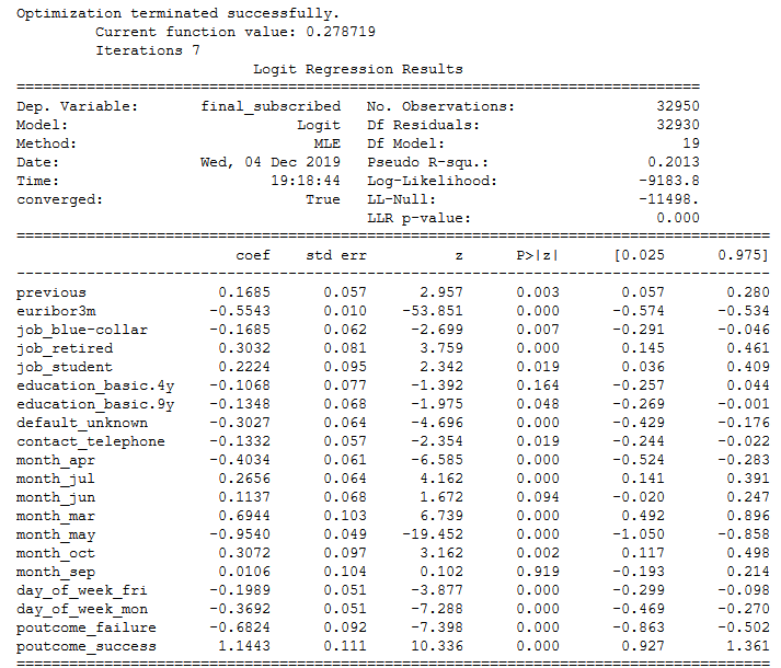
All significant features (here alpha <0.05) are selected and assigned to a new x.
#Here we select just significant features


alpha = 0.05

#Creation of a dataframe with the features just used and the associated p-values
#Filtering this dataframe for p-values < alpha (here 0.05)
df = pd.DataFrame(model_fit.pvalues, columns=['p-value']).reset_index().rename(columns={'index':'features'})
df = df[(df["p-value"] < alpha)]

#Storage of the remaining features in an obejct
filtered_features2 = df['features']

#Creation of a new train and test X
new_train_x2 = new_train_x[filtered_features2]
new_test_x2 = new_test_x[filtered_features2]
6 Logistic Regression with scikit-learn
6.1 Over-sampling using SMOTE
SMOTE is an over-sampling method and stands for Synthetic Minority Over-sampling Technique . What it does is, it creates synthetic (not duplicate) samples of the minority class. Hence making the minority class equal to the majority class. SMOTE does this by selecting similar records and altering that record one column at a time by a random amount within the difference to the neighbouring records.
There are two important points to note here:
SMOTE is only applied to the training data.Because by oversampling only on the training data, none of the information in the test data is being used to create synthetic observations, therefore, no information will bleed from test data into the model training.
Do not use SMOTE before using feature selection methods. Performing variable selection after using SMOTE should be done with some care because most variable selection methods assume that the samples are independent.
columns_x = new_train_x2.columns


sm = SMOTE(random_state=0)
trainX_smote ,trainY_smote = sm.fit_resample(new_train_x2, trainY)

trainX_smote = pd.DataFrame(data=trainX_smote,columns=columns_x)
trainY_smote = pd.DataFrame(data=trainY_smote,columns=['final_subscribed'])
The previously imbalanced dataset is now balanced.
print("Before OverSampling, counts of label '1': {}".format(sum(trainY==1)))
print("Before OverSampling, counts of label '0': {} \n".format(sum(trainY==0)))

print("After OverSampling, counts of label '1':", trainY_smote[(trainY_smote["final_subscribed"] == 1)].shape[0])
print("After OverSampling, counts of label '0':", trainY_smote[(trainY_smote["final_subscribed"] == 0)].shape[0])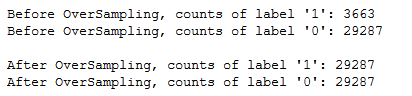
sns.countplot(x='final_subscribed', data=trainY_smote, palette='hls')
print(plt.show())
print("Proportion of no subscription data in oversampled data is ",len(trainY_smote[trainY_smote['final_subscribed']==0])/len(trainX_smote))
print("Proportion of subscription data in oversampled data is ",len(trainY_smote[trainY_smote['final_subscribed']==1])/len(trainX_smote))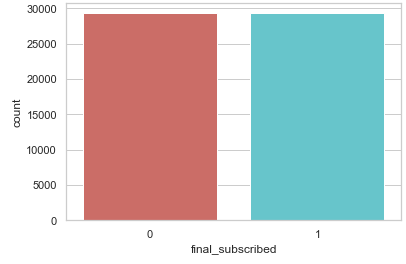
The complete dataset has become bigger:
print('Shape bevore OverSampling:')
print("Number of observations trainX dataset:", new_train_x2.shape[0])
print("Number of observations trainY dataset:", trainY.shape[0])


print('\nShape after OverSampling:')
print("Number of observations trainX_os dataset:", trainX_smote.shape[0])
print("Number of observations trainY_os dataset:", trainY_smote.shape[0])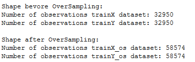
6.2 Model Fitting
After all the selections of the features and creation of the synthetic samples, here again an overview of the train and test predictors as well as the train and test criterion. For a better overview, we assign the objects more descriptive / known names.
trainX_final = trainX_smote
testX_final = new_test_x2
trainY_final = trainY_smote
testY_final = testY
logreg = LogisticRegression()
logreg.fit(trainX_final, trainY_final)
y_pred = logreg.predict(testX_final)Here is a nice overview of the features, their associated coefficients and odds ratios:
coef = pd.DataFrame({'features': trainX_final.columns,
                     'coef': logreg.coef_[0],
                     'odds_ratio': np.exp(logreg.coef_[0])})

coef[['features', 'coef', 'odds_ratio']]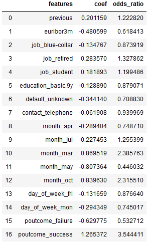
6.3 Model evaluation
6.3.1 Confusion matrix
We usually use a confusion matrix to evaluate classification models. This can be done in python as follows:
confusion_matrix = confusion_matrix(testY_final, y_pred)
print(confusion_matrix)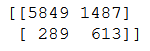
We can also represent the Confusion Matrix with a nice graphic:
fig, ax = plt.subplots(figsize=(6, 6))
ax.matshow(confusion_matrix, cmap=plt.cm.Blues, alpha=0.3)
for i in range(confusion_matrix.shape[0]):
    for j in range(confusion_matrix.shape[1]):
        ax.text(x=j, y=i,s=confusion_matrix[i, j], va='center', ha='center', size='xx-large')

plt.xlabel('Predictions', fontsize=18)
plt.ylabel('Actuals', fontsize=18)
plt.title('Confusion Matrix', fontsize=18)
plt.show()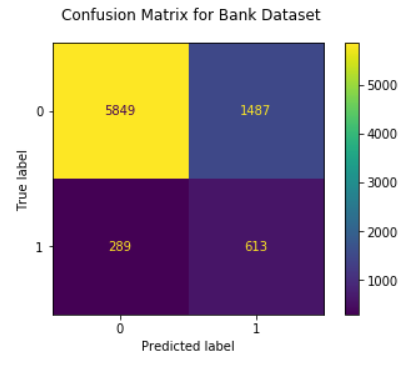
But what does the confusion matrix tell us? To explain this we look at the following graphic:
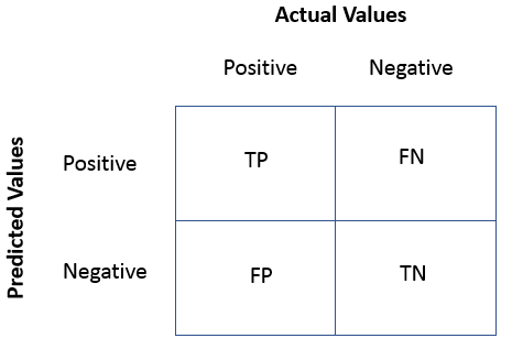
True Positives(TP)= are the cases in which we predicted yes they have subscibed and in reality, they do have subscription.
True Negative(TN)= are the cases in which we predicted no they don’t have subscibed and in reality, they don’t have subscription.
False Positive(FP) = are the cases in which we predicted yes they have subscibed and in reality, they don’t have subscription. This is also known as Type 1 Error.
False Negative(FN)= are the cases in which we predicted no they don’t have subscibed and in reality, they do have subscription. This is also known as the Type 2 Error.
6.3.2 Further metrics
Based on the values from the confusion matrix, the following metrics can be calculated:
print('Accuracy: {:.2f}'.format(accuracy_score(testY_final, y_pred)))
print('Error rate: {:.2f}'.format(1 - accuracy_score(testY_final, y_pred)))
print('Precision: {:.2f}'.format(precision_score(testY_final, y_pred)))
print('Recall: {:.2f}'.format(recall_score(testY_final, y_pred)))
print('f1_score: {:.2f}'.format(f1_score(testY_final, y_pred)))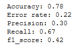
Accuracy is the fraction of predictions our model got right.
Error rate is the fraction of predictions our model got wrong.
The precision is intuitively the ability of the classifier to not label a sample as positive if it is negative.
The recall is intuitively the ability of the classifier to find all the positive samples.
The F1 score can be interpreted as a weighted average of the precision and recall, where an F1 score reaches its best value at 1 and worst score at 0.
6.3.3 ROC / AUC
logit_roc_auc = roc_auc_score(testY_final, logreg.predict(testX_final))
fpr, tpr, thresholds = roc_curve(testY_final, logreg.predict_proba(testX_final)[:,1])
plt.figure()
plt.plot(fpr, tpr, label='Logistic Regression (area = %0.2f)' % logit_roc_auc)
plt.plot([0, 1], [0, 1],'r--')
plt.xlim([0.0, 1.0])
plt.ylim([0.0, 1.05])
plt.xlabel('False Positive Rate')
plt.ylabel('True Positive Rate')
plt.title('Receiver operating characteristic ROC')
plt.legend(loc="lower right")

plt.show()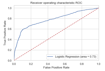
The receiver operating characteristic (ROC) curve is another common tool used with binary classifiers. It shows the tradeoff between sensitivity and specificity. The dotted line represents the ROC curve of a purely random classifier; a good classifier stays as far away from that line as possible. This means that the top left corner of the chart is the “ideal” point - a false positive rate of zero and a true positive rate of one. This is not very realistic, but it means that a larger area under the curve (AUC) is usually better.
We can calculate AUC as follows:
y_pred_proba = logreg.predict_proba(testX_final)[::,1]
roc_auc_score(testY_final, y_pred_proba)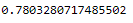
AUC score 1 represents perfect classifier, and 0.5 represents a worthless classifier.
Multiple ROC curves
The library scikit-learn also has a function (plot_roc_curve) that creates such a graph easier and faster. In addition, we have the possibility to compare the performance of several classification algorithms in one graph.
For this purpose, I will again train three different classification algorithms and then compare their performance.
I will explain how the DecisionTreeClassifier or the RandomForestClassifier works in more detail in a later post.
lr = LogisticRegression()
dt = DecisionTreeClassifier()
rf = RandomForestClassifier()
lr.fit(trainX_final, trainY_final)
dt.fit(trainX_final, trainY_final)
rf.fit(trainX_final, trainY_final)disp = plot_roc_curve(lr, testX_final, testY_final)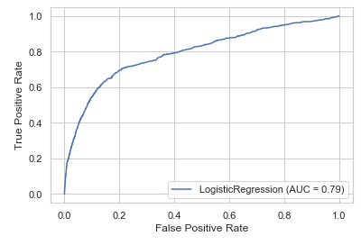
disp = plot_roc_curve(lr, testX_final, testY_final);
plot_roc_curve(dt, testX_final, testY_final, ax=disp.ax_);
plot_roc_curve(rf, testX_final, testY_final, ax=disp.ax_)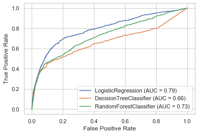
6.3.4 Cross Validation
Another option for model evaluation is the use of Cross Validation (CV).
With CV we try to validate the stability of the machine learning model-how well it would generalize to new data. It needs to be sure that the model has got most of the patterns from the data correct, and its not picking up too much on the noise, or in other words its low on bias and variance.
Here is an overview how Cross Valitation works:
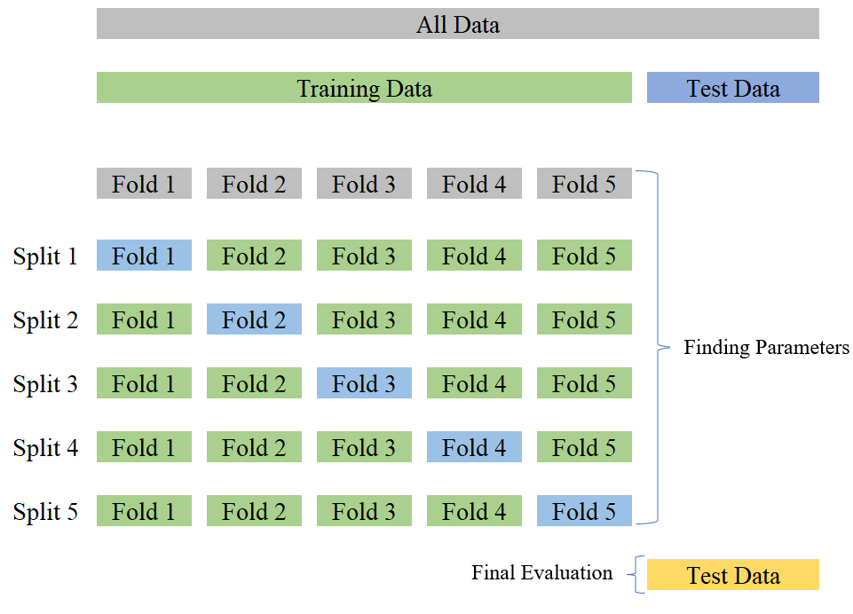
clf = LogisticRegression()
scores = cross_val_score(clf, trainX_final, trainY_final, cv=5)
scores
We see that the accuracy values do not have a high variance. That’s good!
print("Accuracy: %0.2f (+/- %0.2f)" % (scores.mean(), scores.std()))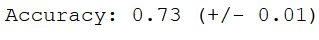
7 Conclusion
The logistic regression was the first classification algorithm that was dealt with in my posts. Although this algorithm is not one of the most complex of its kind, it is often used because of its simplicity and delivers very satisfactory values.
8 Description of the dataframe
Predictors variables:
- age (numeric)
- job (categorical)
- marital (categorical)
- education (categorical)
- default: has credit in default? (categorical: “no”, “yes”, “unknown”)
- housing: has housing loan? (categorical: “no”, “yes”, “unknown”)
- loan: has personal loan? (categorical: “no”, “yes”, “unknown”)
- contact: contact communication type (categorical: “cellular”, “telephone”)
- month: last contact month of year (categorical: “jan”, “feb”, “mar”, …, “nov”, “dec”)
- day_of_week: last contact day of the week (categorical: “mon”, “tue”, “wed”, “thu”, “fri”)
- duration: last contact duration, in seconds (numeric)
- campaign: number of contacts performed during this campaign and for this client (numeric)
- pdays: number of days that passed by after the client was last contacted from a previous campaign (numeric)
- previous: number of contacts performed before this campaign and for this client (numeric)
- poutcome: outcome of the previous marketing campaign (categorical)
- emp.var.rate: employment variation rate (numeric)
- cons.price.idx: consumer price index (numeric)
- cons.conf.idx: consumer confidence index (numeric)
- euribor3m (numeric)
- nr.employed (numeric)
Target variable:
- final subscribed: has the client subscribed a term deposit? (binary: “1”, means “Yes”, “0” means “No”)