- 1 Introduction
- 2 Theoretical Background
- 3 Import the libraries
- 4 XGBoost for Classification
- 5 XGBoost for Regression
- 6 Conclusion
1 Introduction
In my previous post I talked about boosting methods and introduced the algorithms AdaBoost and Gradient Boosting.
There is another boosting algorithm that has become very popular because its performance and predictive power is extremely good. We are talking here about the so-called XGBoost.
For this post I used two different datasets which can be found on the statistics platform “Kaggle”. You can download them from my “GitHub Repository” as well.
I used:
bank.csvfor the Classification part andhouce_prices.csvfor the Regression part
2 Theoretical Background
As we know from the Ensemble Modeling - Boosting post, gradient boosting is one of the most powerful techniques for building predictive models. XGBoost is an efficient implementation of gradient boosting for classification and regression problems.
Some useful links:
Introduction to Gradient Boosting
The Gradient Boosting algorithm involves three elements:
- A loss function to be optimized, such as cross entropy for classification or mean squared error for regression problems.
- A weak learner to make predictions, such as a greedily constructed decision tree.
- An additive model, used to add weak learners to minimize the loss function.
New weak learners are added to the model in an effort to correct the residual errors of all previous trees. The result is a powerful predictive modeling algorithm.
Introduction to XGBoost
XGBoost is an implementation of gradient boosted decision trees designed for speed and performance.
XGBoost stands for
- eXtreme
- Gradient
- Boosting
In addition to supporting all key variations of the technique, the real interest is the speed provided by the careful engineering of the implementation, including:
- Parallelization of tree construction using all of your CPU cores during training.
- Distributed Computing for training very large models using a cluster of machines.
- Out-of-Core Computing for very large datasets that don’t fit into memory.
- Cache Optimization of data structures and algorithms to make best use of hardware.
The advantage of XGBoost over other boosting algorithms is clearly the speed at which it works.
Getting Started
The machine learning library Scikit-Learn supports different implementations of gradient boosting classifiers, including XGBoost. You can install it using pip, as follows:
pip install xgboost
3 Import the libraries
import pandas as pd
import numpy as np

from sklearn.model_selection import train_test_split
from matplotlib import pyplot as plt
from matplotlib import pyplot

from sklearn.metrics import accuracy_score
from sklearn.metrics import mean_squared_error

from sklearn.model_selection import GridSearchCV
from sklearn.model_selection import TimeSeriesSplit


import xgboost as xgb
from xgboost import plot_importance
from xgboost import XGBClassifier
from xgboost import XGBRegressor

import warnings
warnings.filterwarnings("ignore")
4 XGBoost for Classification
4.1 Load the bank dataset
bank = pd.read_csv("bank.csv", sep=";")
bank.head()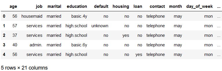
4.2 Pre-process the bank dataset
safe_y = bank[['y']]

col_to_exclude = ['y']
bank = bank.drop(col_to_exclude, axis=1)

#Just select the categorical variables
cat_col = ['object']
cat_columns = list(bank.select_dtypes(include=cat_col).columns)
cat_data = bank[cat_columns]
cat_vars = cat_data.columns

#Create dummy variables for each cat. variable
for var in cat_vars:
    cat_list = pd.get_dummies(bank[var], prefix=var)
    bank=bank.join(cat_list)


data_vars=bank.columns.values.tolist()
to_keep=[i for i in data_vars if i not in cat_vars]

#Create final dataframe
bank_final=bank[to_keep]

bank = pd.concat([bank_final, safe_y], axis=1)
bank.head()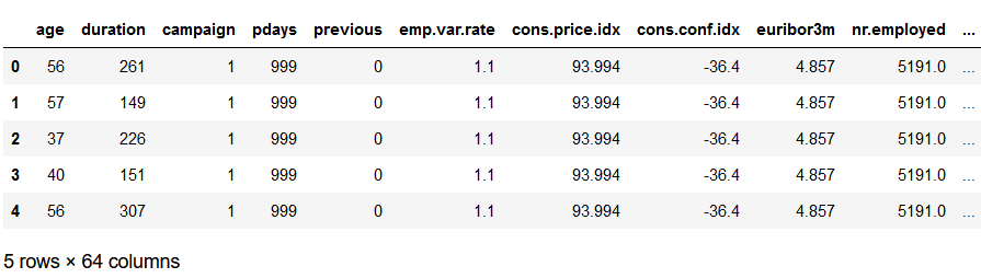
x = bank.drop('y', axis=1)
y = bank['y']

trainX, testX, trainY, testY = train_test_split(x, y, test_size = 0.2)
4.3 Fit the Model
I use objective=‘binary:logistic’ function because I train a classifier which handles only two classes.
If you have a multi label classification problem use objective=‘multi:softmax’ or ‘multi:softprob’ as described here: Learning Task Parameters.
xgb = XGBClassifier(objective= 'binary:logistic')
xgb.fit(trainX, trainY)
4.4 Evaluate the Model
preds_train = xgb.predict(trainX)
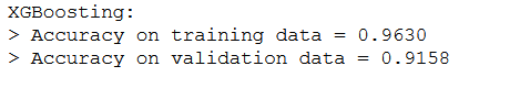
preds_test = xgb.predict(testX)print('XGBoosting:\n> Accuracy on training data = {:.4f}\n> Accuracy on validation data = {:.4f}'.format(
accuracy_score(y_true=trainY, y_pred=preds_train),
accuracy_score(y_true=testY, y_pred=preds_test)
))
4.5 Monitor Performance and Early Stopping
XGBoost can evaluate and report on the performance on a test set during model training.
For example, we can report on the binary classification error rate (error) on a standalone test set (eval_set) while training an XGBoost model as follows:
eval_set = [(testX, testY)]
xgb.fit(trainX, trainY, eval_metric="error", eval_set=eval_set, verbose=True)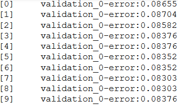
For multiple classification problems use eval_metric=“merror”.
To get a better overview of the available parameters, check out XGBoost Parameters.
Subsequently, we will use this information to interrupt the model training as soon as no significant improvement takes place. We can do this by setting the early_stopping_rounds parameter when calling model.fit() to the number of iterations that no improvement is seen on the validation dataset before training is stopped.
xgb_es = XGBClassifier(objective= 'binary:logistic')

eval_set = [(testX, testY)]
xgb_es.fit(trainX, trainY, early_stopping_rounds=7, eval_metric="error", eval_set=eval_set, verbose=True)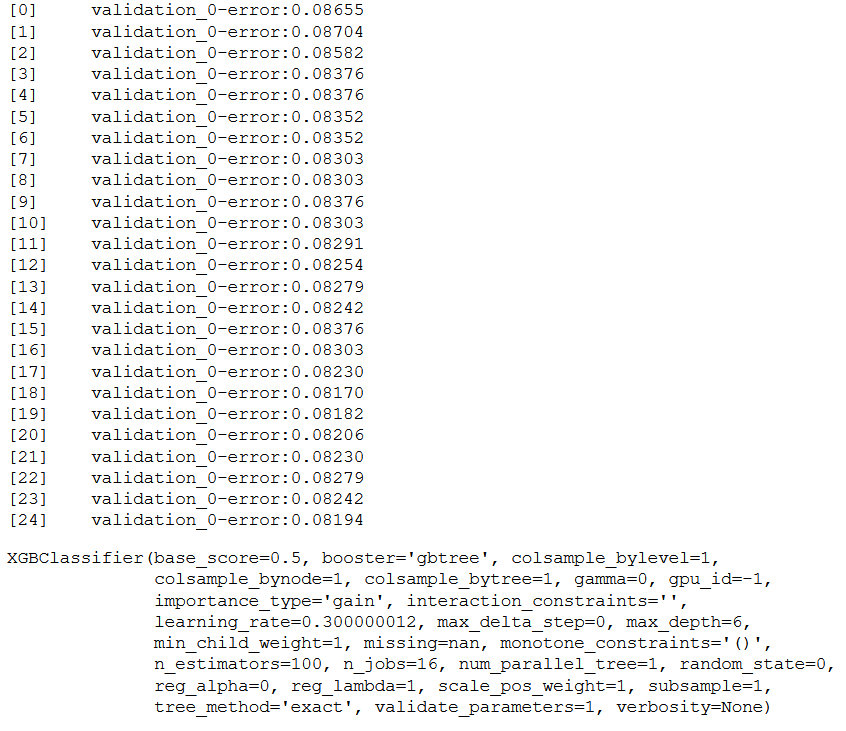
preds_train = xgb_es.predict(trainX)
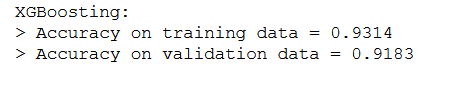
preds_test = xgb_es.predict(testX)print('XGBoosting:\n> Accuracy on training data = {:.4f}\n> Accuracy on validation data = {:.4f}'.format(
accuracy_score(y_true=trainY, y_pred=preds_train),
accuracy_score(y_true=testY, y_pred=preds_test)
))
4.6 Xgboost Built-in Feature Importance
Another general advantage of using ensembles of decision tree methods like gradient boosting (which has not yet come up in my boosting post) is that they can automatically provide estimates of feature importance from a trained model.
A trained XGBoost model automatically calculates feature importance on your predictive modeling problem.
4.6.1 Get Feature Importance of all Features
print(xgb_es.feature_importances_)
print()
print('Length of feature_importances_ list: ' + str(len(xgb_es.feature_importances_)))
print()
print('Number of predictors in trainX: ' + str(trainX.shape[1]))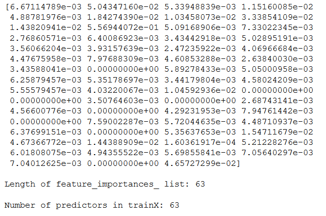
We can directly plot the feature importance with plot_importance.
# plot feature importance
plot_importance(xgb_es)
pyplot.show()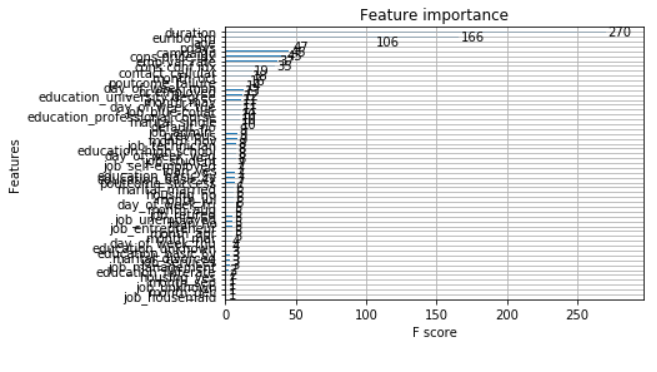
Since this overview is extremely poor, let’s look at just the best 10 features:
feature_names = trainX.columns

feature_importance_df = pd.DataFrame(xgb_es.feature_importances_, feature_names)
feature_importance_df = feature_importance_df.reset_index()
feature_importance_df.columns = ['Feature', 'Importance']
feature_importance_df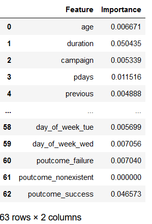
feature_importance_df_top_10 = feature_importance_df.sort_values(by='Importance', ascending=False).head(10)
feature_importance_df_top_10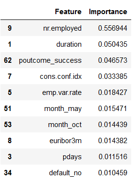
plt.barh(feature_importance_df_top_10.Feature, feature_importance_df_top_10.Importance)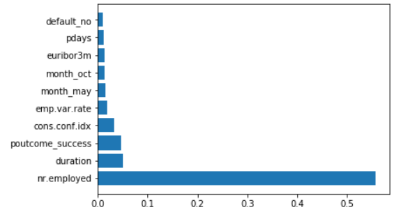
4.6.2 Get the feature importance of all the features the model has retained
Previously, we saw the importance that the XGBoost algorithm assigns to each predictor. XGBoost automatically takes this information for effective model training. This means that not all variables are included in the training.
features_selected_from_XGBoost = xgb_es.get_booster().get_score(importance_type='gain')
keys = list(features_selected_from_XGBoost.keys())
values = list(features_selected_from_XGBoost.values())

features_selected_from_XGBoost = pd.DataFrame(data=values,
                                              index=keys,
                                              columns=["Importance"]).sort_values(by = "Importance",
                                                                             ascending=False)
features_selected_from_XGBoost.plot(kind='barh')

print()
print('Length of remaining predictors after XGB: ' + str(len(features_selected_from_XGBoost)))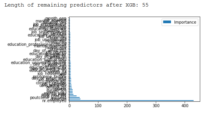
So what variables were not considered? Quite simply: all those that have been assigned an Importance Score of 0. Let’s filter our feature_importance_df for score == 0.
print(feature_importance_df[(feature_importance_df["Importance"] == 0)])
print()
print('Length of features with Importance = zero:  ' + str(feature_importance_df[(feature_importance_df["Importance"] == 0)].shape[0] ))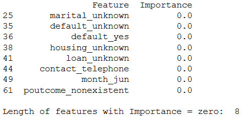
The following step can be considered superfluous, but I’ll do it anyway and get the 10 best features that the model has kept. These should also be the same as in the last step in chapter 4.6.1.
top_10_of_retained_features_from_model = features_selected_from_XGBoost.sort_values(by='Importance', ascending=False).head(10)
top_10_of_retained_features_from_model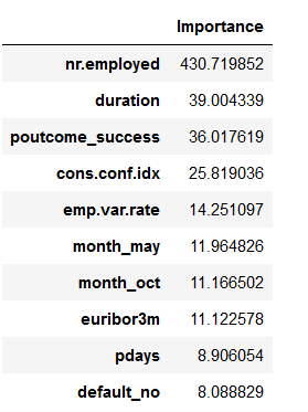
plt.barh(top_10_of_retained_features_from_model.index, top_10_of_retained_features_from_model.Importance)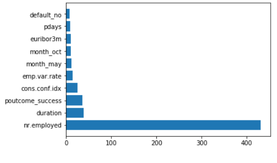
4.7 Grid Search
xgb_grid = XGBClassifier(objective= 'binary:logistic')parameters = {
'max_depth': range (2, 10, 1),
'colsample_bytree': [0.6, 0.8, 1.0],
'gamma': [0.5, 1, 1.5],
'n_estimators': range(60, 220, 40),
'learning_rate': [0.0001, 0.001, 0.01, 0.1, 0.2]}Grid Search may take an extremely long time to calculate all possible given combinations of parameters. With XGBoost we have the comfortable situation of using early stopping. This function can also be implemented in Grid Search.
fit_params={"early_stopping_rounds":10,
            "eval_metric" : "rmse",
            "eval_set" : [[testX, testY]]}
For scoring I have chosen ‘neg_log_loss’ here. However, a number of other parameters can also be used, see here: Scoring parameter.
Set verbose=1 if you want to receive information about the processing status of grid search. As you can see from the output below, there are 1440 possible combinations for the defined parameter values, which are calculated by GridSearch (83345 = 1,440). Add to this the number of cross-validations (cv=5) resulting in a total number of 7,200 fits (1,440*5).
These calculations would take a long time even with a good computer. I therefore strongly recommend to use early stopping also when using GridSearch.
cv = 5

grid_search = GridSearchCV(
    estimator=xgb_grid,
    param_grid=parameters,
    scoring = 'neg_log_loss',
    n_jobs = -1,
    cv = TimeSeriesSplit(n_splits=cv).get_n_splits([trainX, trainY]),
    verbose=1)

xgb_grid_model = grid_search.fit(trainX, trainY, **fit_params)
print('Best Parameter:')
print(xgb_grid_model.best_params_)
print()
print('------------------------------------------------------------------')
print()
print(xgb_grid_model.best_estimator_)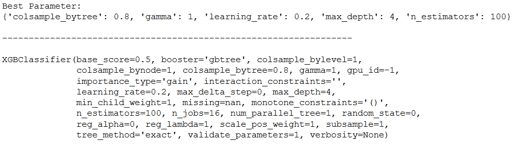
preds_train = xgb_grid_model.predict(trainX)
preds_test = xgb_grid_model.predict(testX)

print('XGBoosting with GridSearch:\n> Accuracy on training data = {:.4f}\n> Accuracy on validation data = {:.4f}'.format(
    accuracy_score(y_true=trainY, y_pred=preds_train),
    accuracy_score(y_true=testY, y_pred=preds_test)
))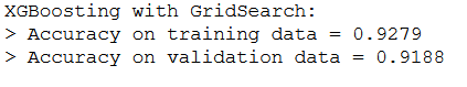
Yeah, we were able to increase the prediction accuracy again.
5 XGBoost for Regression
5.1 Load the house_prices dataset
house = pd.read_csv("houce_prices.csv")
house = house.drop(['zipcode', 'lat', 'long', 'date', 'id'], axis=1)
house.head()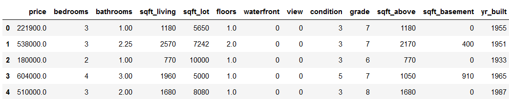
x = house.drop('price', axis=1)
y = house['price']
trainX, testX, trainY, testY = train_test_split(x, y, test_size = 0.2)
5.2 Fit the Model
xgb = XGBRegressor(objective= 'reg:linear')
xgb.fit(trainX, trainY)
5.3 Evaluate the Model
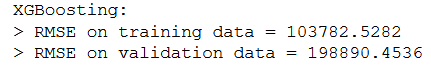
preds_train = xgb.predict(trainX)
preds_test = xgb.predict(testX)
print('XGBoosting:\n> RMSE on training data = {:.4f}\n> RMSE on validation data = {:.4f}'.format(
np.sqrt(mean_squared_error(y_true=trainY, y_pred=preds_train)),
np.sqrt(mean_squared_error(y_true=testY, y_pred=preds_test))
))
5.4 Early Stopping
xgb_es = XGBRegressor(objective= 'reg:linear')
eval_set = [(testX, testY)]
xgb_es.fit(trainX, trainY, early_stopping_rounds=20, eval_metric="rmse", eval_set=eval_set, verbose=True)preds_train = xgb_es.predict(trainX)
preds_test = xgb_es.predict(testX)print('XGBoosting:\n> RMSE on training data = {:.4f}\n> RMSE on validation data = {:.4f}'.format(
np.sqrt(mean_squared_error(y_true=trainY, y_pred=preds_train)),
np.sqrt(mean_squared_error(y_true=testY, y_pred=preds_test))
))
5.5 Feature Importance
# plot feature importance
plot_importance(xgb_es)
pyplot.show()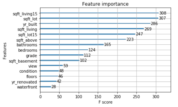
5.6 Grid Search
xgb_grid = XGBRegressor(objective= 'reg:linear')parameters = {
'n_estimators': [400, 700, 1000],
'colsample_bytree': [0.7, 0.8],
'max_depth': [15,20,25],
'reg_alpha': [1.1, 1.2, 1.3],
'reg_lambda': [1.1, 1.2, 1.3],
'subsample': [0.7, 0.8, 0.9]}fit_params={"early_stopping_rounds":10,
"eval_metric" : "rmse",
"eval_set" : [[testX, testY]]}cv = 5
grid_search = GridSearchCV(
estimator=xgb_grid,
param_grid=parameters,
scoring = 'neg_mean_squared_error',
n_jobs = -1,
cv = TimeSeriesSplit(n_splits=cv).get_n_splits([trainX, trainY]),
verbose=1)
xgb_grid_model = grid_search.fit(trainX, trainY, **fit_params) 
print('Best Parameter:')
print(xgb_grid_model.best_params_)
print()
print('------------------------------------------------------------------')
print()
print(xgb_grid_model.best_estimator_)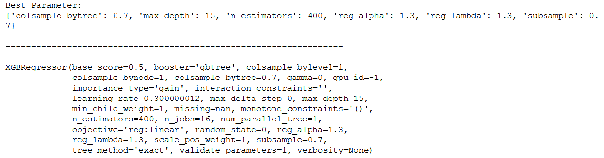
preds_train = xgb_grid_model.predict(trainX)
preds_test = xgb_grid_model.predict(testX)
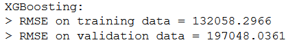
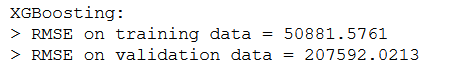
print('XGBoosting:\n> RMSE on training data = {:.4f}\n> RMSE on validation data = {:.4f}'.format(
    np.sqrt(mean_squared_error(y_true=trainY, y_pred=preds_train)),
    np.sqrt(mean_squared_error(y_true=testY, y_pred=preds_test))
))
6 Conclusion
That’s it. I gave a comprehensive theoretical introduction to gradient boosting and went into detail about XGBoost and its use. I showed how the XGBoost algorithm can be used to solve classification and regression problems.
Comparing the performance with the results of the other ensemble algorithms:
we see that the XG Boost performs better. This is the reason of its great popularity. The same applies when using the XGBoost for regressions.
One final note:
You can also use XG Boost for time series analysis. See this post of mine about this: XGBoost for Univariate Time Series