1 Introduction
2 Import the libraries and the data
3 Definition of required functions
4 Train Test Split
5 Create Time Series Features
6 Fit the Model
7 Get Feature Importance
8 Forecast And Evaluation
9 Look at Worst and Best Predicted Days
10 Grid Search
11 Conclusion

1 Introduction

Now I have written a few posts in the recent past about Time Series and Forecasting. But I didn’t want to deprive you of a very well-known and popular algorithm: XGBoost

The exact functionality of this algorithm and an extensive theoretical background I have already given in this post: Ensemble Modeling - XGBoost.

For this post the dataset PJME_hourly from the statistic platform “Kaggle” was used. You can download it from my “GitHub Repository”.

2 Import the libraries and the data

import pandas as pd
import numpy as np

from matplotlib import pyplot as plt
from sklearn import metrics

from pmdarima.model_selection import train_test_split as time_train_test_split

from xgboost import XGBRegressor
from xgboost import plot_importance

import warnings
warnings.filterwarnings("ignore")

The dataset is about the Hourly Energy Consumption from PJM Interconnection LLC (PJM) in Megawatts.

pjme = pd.read_csv('PJME_hourly.csv')

# Convert column Datetime to data format datetime
pjme['Datetime'] = pd.to_datetime(pjme['Datetime'])

# Make sure that you have the correct order of the times 
pjme = pjme.sort_values(by='Datetime', ascending=True)

# Set Datetime as index
pjme = pjme.set_index('Datetime')
pjme

3 Definition of required functions

def create_features(df, target_variable):
    """
    Creates time series features from datetime index
    
    Args:
        df (float64): Values to be added to the model incl. corresponding datetime
                      , numpy array of floats
        target_variable (string): Name of the target variable within df   
    
    Returns:
        X (int): Extracted values from datetime index, dataframe
        y (int): Values of target variable, numpy array of integers
    """
    df['date'] = df.index
    df['hour'] = df['date'].dt.hour
    df['dayofweek'] = df['date'].dt.dayofweek
    df['quarter'] = df['date'].dt.quarter
    df['month'] = df['date'].dt.month
    df['year'] = df['date'].dt.year
    df['dayofyear'] = df['date'].dt.dayofyear
    df['dayofmonth'] = df['date'].dt.day
    df['weekofyear'] = df['date'].dt.weekofyear
    
    X = df[['hour','dayofweek','quarter','month','year',
           'dayofyear','dayofmonth','weekofyear']]
    if target_variable:
        y = df[target_variable]
        return X, y
    return X

def mean_absolute_percentage_error_func(y_true, y_pred):
    '''
    Calculate the mean absolute percentage error as a metric for evaluation
    
    Args:
        y_true (float64): Y values for the dependent variable (test part), numpy array of floats 
        y_pred (float64): Predicted values for the dependen variable (test parrt), numpy array of floats
    
    Returns:
        Mean absolute percentage error 
    '''    
    y_true, y_pred = np.array(y_true), np.array(y_pred)
    return np.mean(np.abs((y_true - y_pred) / y_true)) * 100

def timeseries_evaluation_metrics_func(y_true, y_pred):
    '''
    Calculate the following evaluation metrics:
        - MSE
        - MAE
        - RMSE
        - MAPE
        - R²
    
    Args:
        y_true (float64): Y values for the dependent variable (test part), numpy array of floats 
        y_pred (float64): Predicted values for the dependen variable (test parrt), numpy array of floats
    
    Returns:
        MSE, MAE, RMSE, MAPE and R² 
    '''    
    #print('Evaluation metric results: ')
    print(f'MSE is : {metrics.mean_squared_error(y_true, y_pred)}')
    print(f'MAE is : {metrics.mean_absolute_error(y_true, y_pred)}')
    print(f'RMSE is : {np.sqrt(metrics.mean_squared_error(y_true, y_pred))}')
    print(f'MAPE is : {mean_absolute_percentage_error_func(y_true, y_pred)}')
    print(f'R2 is : {metrics.r2_score(y_true, y_pred)}',end='\n\n')

4 Train Test Split

X = pjme['PJME_MW']

# Test Size = 20%
train_pjme, test_pjme = time_train_test_split(X, test_size=int(len(pjme)*0.2))

train_pjme = pd.DataFrame(train_pjme)
test_pjme = pd.DataFrame(test_pjme)

Overview_Train_Test_Data = test_pjme \
    .rename(columns={'PJME_MW': 'TEST SET'}) \
    .join(train_pjme.rename(columns={'PJME_MW': 'TRAINING SET'}), how='outer') \
    .plot(figsize=(15,5), title='Overview Train Test Data', style='.')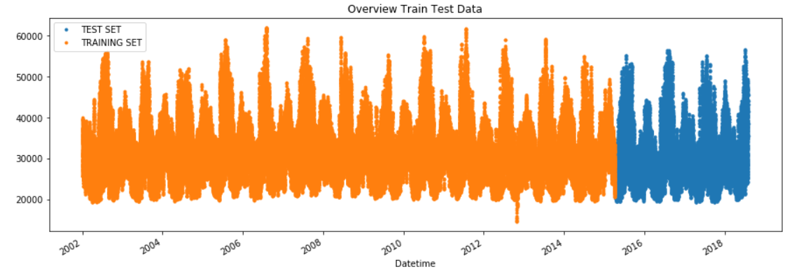

5 Create Time Series Features

train_pjme_copy = train_pjme.copy()
test_pjme_copy = test_pjme.copy()

trainX, trainY = create_features(train_pjme_copy, target_variable='PJME_MW')
testX, testY = create_features(test_pjme_copy, target_variable='PJME_MW')

trainX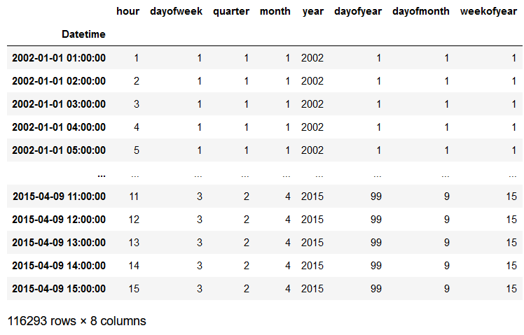

trainY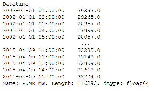

6 Fit the Model

xgb = XGBRegressor(objective= 'reg:linear', n_estimators=1000)
xgb

xgb.fit(trainX, trainY,
        eval_set=[(trainX, trainY), (testX, testY)],
        early_stopping_rounds=50,
        verbose=False) # Change verbose to True if you want to see it train

7 Get Feature Importance

feature_importance = plot_importance(xgb, height=0.9)
feature_importance

8 Forecast And Evaluation

predicted_results = xgb.predict(testX)
predicted_results

timeseries_evaluation_metrics_func(testY, predicted_results)

plt.figure(figsize=(13,8))
plt.plot(list(testY))
plt.plot(list(predicted_results))
plt.title("Actual vs Predicted")
plt.ylabel("PJME_MW")
plt.legend(('Actual','predicted'))
plt.show()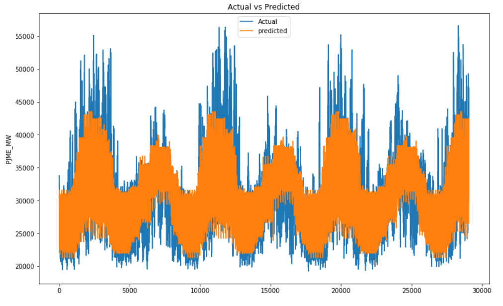

test_pjme['Prediction'] = predicted_results
pjme_all = pd.concat([test_pjme, train_pjme], sort=False)
pjme_all = pjme_all.rename(columns={'PJME_MW':'Original_Value'})

Overview_Complete_Data_And_Prediction = pjme_all[['Original_Value','Prediction']].plot(figsize=(15, 5))

Let’s have a look at the smallest date for which predictions were made.

print('Smallest date for which predictions were made: ' )
print(str(test_pjme.index.min()))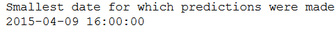

# Plot the forecast with the actuals for Mai
f, ax = plt.subplots(1)
f.set_figheight(5)
f.set_figwidth(13)
Overview_Mai_2015 = pjme_all[['Prediction','Original_Value']].plot(ax=ax,
                                                                   style=['-','.'])
ax.set_xbound(lower='2015-05-01', upper='2015-06-01')
ax.set_ylim(0, 60000)
plot = plt.suptitle('Mai 2015 Forecast vs Actuals')

# Plot the forecast with the actuals for the first week of Mai
f, ax = plt.subplots(1)
f.set_figheight(5)
f.set_figwidth(13)
Overview_Mai_2015 = pjme_all[['Prediction','Original_Value']].plot(ax=ax,
                                                                   style=['-','.'])
ax.set_xbound(lower='2015-05-01', upper='2015-05-08')
ax.set_ylim(0, 60000)
plot = plt.suptitle('First Week of Mai 2015 Forecast vs Actuals')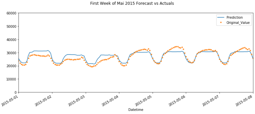

9 Look at Worst and Best Predicted Days

# Copy test_pjme
Worst_Best_Pred = test_pjme.copy()
Worst_Best_Pred = Worst_Best_Pred.reset_index()

# Generate error and absolut error values for the predictions made
Worst_Best_Pred['error'] = Worst_Best_Pred['PJME_MW'] - Worst_Best_Pred['Prediction']
Worst_Best_Pred['abs_error'] = Worst_Best_Pred['error'].apply(np.abs)

# Extract Year, Month, Day of Month
Worst_Best_Pred['year'] = Worst_Best_Pred['Datetime'].dt.year
Worst_Best_Pred['month'] = Worst_Best_Pred['Datetime'].dt.month
Worst_Best_Pred['dayofmonth'] = Worst_Best_Pred['Datetime'].dt.day

Worst_Best_Pred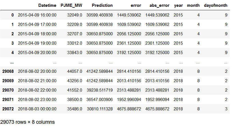

# Group error by days
error_by_day = Worst_Best_Pred.groupby(['year','month','dayofmonth']) \
    .mean()[['PJME_MW','Prediction','error','abs_error']]

error_by_day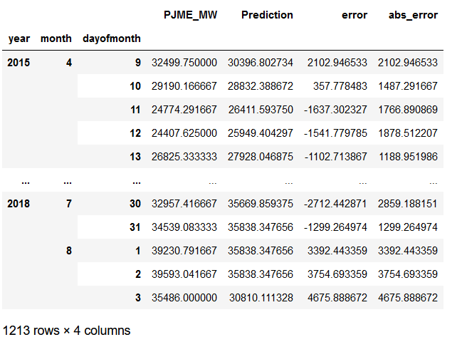

# Worst absolute predicted days
error_by_day.sort_values('abs_error', ascending=False).head(10)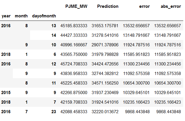

# Best predicted days
error_by_day.sort_values('abs_error', ascending=True).head(10)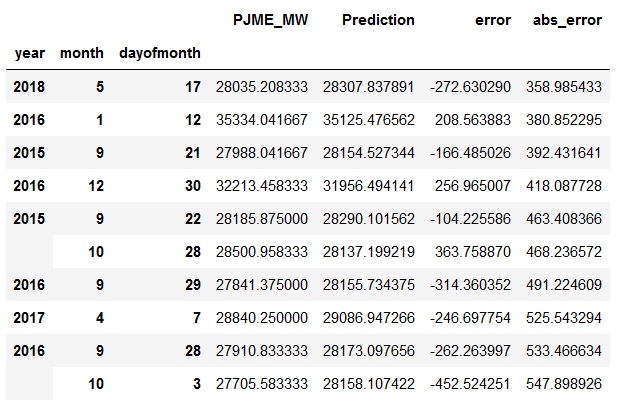

# Plot the forecast with the actuals for Mai
f, ax = plt.subplots(1)
f.set_figheight(5)
f.set_figwidth(13)
Overview_Mai_2015 = pjme_all[['Prediction','Original_Value']].plot(ax=ax,
                                                                   style=['-','.'])
ax.set_xbound(lower='2016-08-13', upper='2016-08-14')
ax.set_ylim(0, 60000)
plot = plt.suptitle('13 Aug, 2016 - Worst Predicted Day')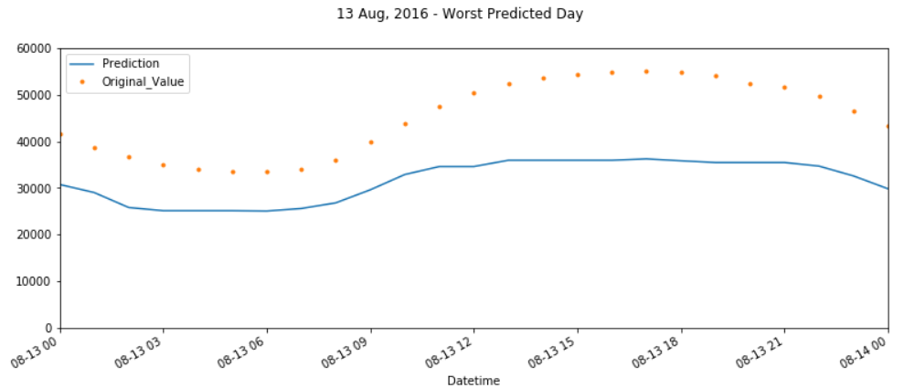

# Plot the forecast with the actuals for Mai
f, ax = plt.subplots(1)
f.set_figheight(5)
f.set_figwidth(13)
Overview_Mai_2015 = pjme_all[['Prediction','Original_Value']].plot(ax=ax,
                                                                   style=['-','.'])
ax.set_xbound(lower='2018-05-17', upper='2018-05-18')
ax.set_ylim(0, 60000)
plot = plt.suptitle('17 Mai, 2018 - Best Predicted Day')

10 Grid Search

If you want, you can try to increase the result and the prediction accuracy by using GridSearch. Here is the necessary syntax for it. I have not run these functions but feel free to do so.

from sklearn.model_selection import GridSearchCV
from sklearn.model_selection import TimeSeriesSplit

xgb_grid = XGBRegressor(objective= 'reg:linear')

parameters = {
    'n_estimators': [700, 1000, 1400],
    'colsample_bytree': [0.7, 0.8],
    'max_depth': [15,20,25],
    'reg_alpha': [1.1, 1.2, 1.3],
    'reg_lambda': [1.1, 1.2, 1.3],
    'subsample': [0.7, 0.8, 0.9]}

fit_params={"early_stopping_rounds":50, 
            "eval_metric" : "rmse", 
            "eval_set" : [[testX, testY]]}

cv = 5

grid_search = GridSearchCV(
    estimator=xgb_grid,
    param_grid=parameters,
    scoring = 'neg_mean_squared_error',
    n_jobs = -1,
    cv = TimeSeriesSplit(n_splits=cv).get_n_splits([trainX, trainY]),
    verbose=1)

xgb_grid_model = grid_search.fit(trainX, trainY, **fit_params)

print('Best Parameter:')
print(xgb_grid_model.best_params_) 
print()
print('------------------------------------------------------------------')
print()
print(xgb_grid_model.best_estimator_)

11 Conclusion

In this post I showed how to make Time Series Forcasts with the XG Boost.

Time Series Analysis - XGBoost for Univariate Time Series