1 Introduction
2 Loading the libraries
3 Introducing PCA
4 PCA in general
5 Randomized PCA
6 Incremental PCA
7 Kernel PCA
8 Tuning Hyperparameters
9 Conclusion

1 Introduction

After the various methods of cluster analysis “Cluster Analysis” have been presented in various publications, we now come to the second category in the area of unsupervised machine learning: Dimensionality Reduction

The areas of application of dimensionality reduction are widely spread within machine learning. Here are some applications of Dimensionality Reduction:

Pre-processing / Feature engineering
Noise reduction
Generating plausible artificial datasets
Financial modelling / risk analysis

For this post the datasets Auto-mpg and MNIST from the statistic platform “Kaggle” were used. A copy of the records is available at my “GitHub Repository” and here: https://drive.google.com/open?id=1Bfquk0uKnh6B3Yjh2N87qh0QcmLokrVk.

2 Loading the libraries

import pandas as pd
import numpy as np

from sklearn.preprocessing import StandardScaler
import matplotlib.pyplot as plt

# Chapter 4&5
from sklearn.decomposition import PCA

# Chapter 6
from sklearn.decomposition import IncrementalPCA

# Chapter 7
from sklearn.decomposition import KernelPCA
from sklearn.datasets import make_swiss_roll

from mpl_toolkits.mplot3d import Axes3D
from pydiffmap import diffusion_map as dm
from pydiffmap.visualization import data_plot

# Chapter 8
from sklearn.model_selection import GridSearchCV
from sklearn.linear_model import LogisticRegression
from sklearn.pipeline import Pipeline
from sklearn.datasets import make_moons
from sklearn.model_selection import train_test_split

3 Introducing PCA

PCA is a commonly used and very effective dimensionality reduction technique, which often forms a pre-processing stage for a number of machine learning models and techniques.

In a nutshell: PCA reduces the sparsity in the dataset by separating the data into a series of components where each component represents a source of information within the data.

As its name suggests, the first principal component produced in PCA, comprises the majority of information or variance within the data. With each subsequent component, less information, but more subtlety, is contributed to the compressed data.

This post is intended to serve as an introduction to PCA in general. In two further publications, the two main uses of the PCA:

PCA for visualization
PCA for speed up machine learning algorithms

are to be presented separately in detail.

4 PCA in general

For the demonstration of PCA in general we’ll load the cars dataset:

cars = pd.read_csv('auto-mpg.csv')
cars["horsepower"] = pd.to_numeric(cars.horsepower, errors='coerce')
cars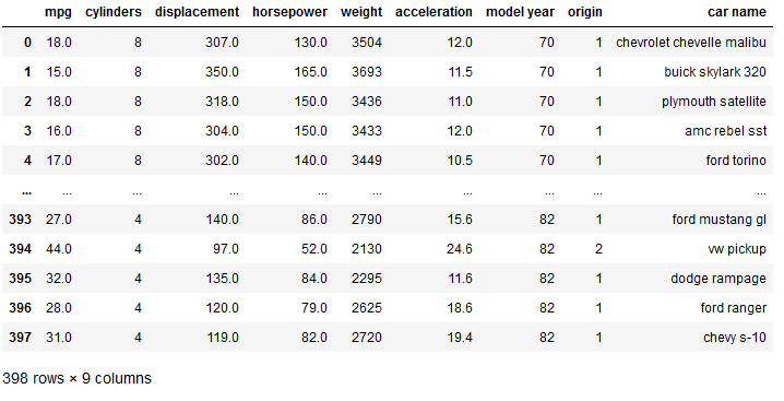

For further use, we throw out all missing values from the data set, split the data set and standardize all predictors.

cars=cars.dropna()

X = cars.drop(['car name'], axis=1)
Y = cars['car name']

sc = StandardScaler()

X = X.values
X_std =  sc.fit_transform(X)

With the following calculations we can see how much variance the individual main components explain within the data set.

cov_matrix = np.cov(X_std.T)

eigenvalues, eigenvectors = np.linalg.eig(cov_matrix)

tot = sum(eigenvalues)
var_explained = [(i / tot) for i in sorted(eigenvalues, reverse=True)] 
cum_var_exp = np.cumsum(var_explained)

plt.bar(range(1,len(var_explained)+1), var_explained, alpha=0.5, align='center', label='individual explained variance')
plt.step(range(1,len(var_explained)+1),cum_var_exp, where= 'mid', label='cumulative explained variance')
plt.ylabel('Explained variance ratio')
plt.xlabel('Principal components')
plt.legend(loc = 'best')
plt.show()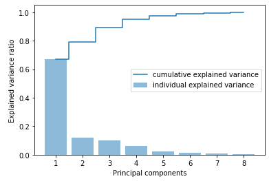

As we can see, it is worth using the first two main components, as together they already explain 80% of the variance.

pca = PCA(n_components = 2)
pca.fit(X_std)
x_pca = pca.transform(X_std)

pca.explained_variance_ratio_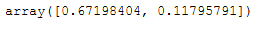

For those who are too lazy to add that up in their heads:

pca.explained_variance_ratio_.sum()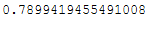

In the previous step, we specified how many main components the PCA should calculated and then asked how much variance these components explained.

We can also approach this process the other way around and tell the PCA how much variance we would like to have explained.

We do this so (for 95% variance):

pca = PCA(n_components = 0.95)
pca.fit(X_std)
x_pca = pca.transform(X_std)

pca.n_components_

4 main components were necessary to achieve 95% variance explanation.

5 Randomized PCA

PCA is mostly used for very large data sets with many variables in order to make them clearer and easier to interpret. This can lead to a very high computing power and long waiting times. Randomized PCA can be used to reduce the calculation time. To do this, simply set the parameter svd_solver to ‘randomized’. In the following example you can see the saving in computing time. This example is carried out with the MNIST data set.

mnist = pd.read_csv('mnist_train.csv')
X = mnist.drop(['label'], axis=1)
sc = StandardScaler()
X = X.values
X_std =  sc.fit_transform(X)
print(X_std.shape)

import time

start = time.time()

pca = PCA(n_components = 200)
pca.fit(X_std)
x_pca = pca.transform(X_std)


end = time.time()
print()
print('Calculation time: ' + str(end - start) + ' seconds')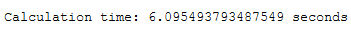

pca_time = end - start

import time

start = time.time()

rnd_pca = PCA(n_components = 200, svd_solver='randomized')
rnd_pca.fit(X_std)
x_rnd_pca = rnd_pca.transform(X_std)

end = time.time()
print()
print('Calculation time: ' + str(end - start) + ' seconds')

rnd_pca_time = end - start

diff = pca_time - rnd_pca_time
diff

procentual_decrease = ((pca_time - rnd_pca_time) / pca_time) * 100
print('Procentual decrease of: ' + str(round(procentual_decrease, 2)) + '%')

6 Incremental PCA

In some cases the data set may be too large to be able to perform a principal component analysis all at once. The Incremental PCA is available for these cases:

With n_batches we determine how much data should always be loaded at once.

n_batches = 100

inc_pca = IncrementalPCA(n_components = 100)
for X_batch in np.array_split(X_std, n_batches):
    inc_pca.partial_fit(X_batch)

inc_pca.explained_variance_ratio_.sum()

7 Kernel PCA

Now we know all too well from practice that some data cannot be linearly separable. Like this one for example:

X, color = make_swiss_roll(n_samples = 1000)
swiss_roll = X
swiss_roll.shape

plt.scatter(swiss_roll[:, 0], swiss_roll[:, 1], c=color)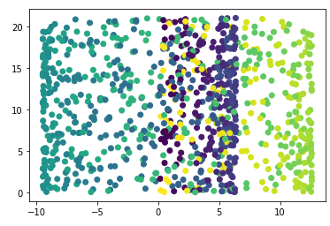

Not really nice to look at. But we can do better.

neighbor_params = {'n_jobs': -1, 'algorithm': 'ball_tree'}

mydmap = dm.DiffusionMap.from_sklearn(n_evecs=2, k=200, epsilon='bgh', alpha=1.0, neighbor_params=neighbor_params)
# fit to data and return the diffusion map.
dmap = mydmap.fit_transform(swiss_roll)

data_plot(mydmap, dim=3, scatter_kwargs = {'cmap': 'Spectral'})
plt.show()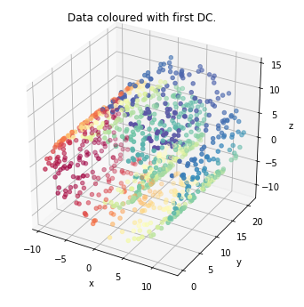

Let’s use some PCA models with different kernels and have a look at how they will perform.

linear_pca = KernelPCA(n_components = 2, kernel='linear')

linear_pca.fit(swiss_roll)

X_reduced_linear = linear_pca.transform(swiss_roll)

X_reduced_linear.shape

plt.scatter(X_reduced_linear[:, 0], X_reduced_linear[:, 1], c = color, cmap=plt.cm.Spectral)
plt.title("Linear kernel")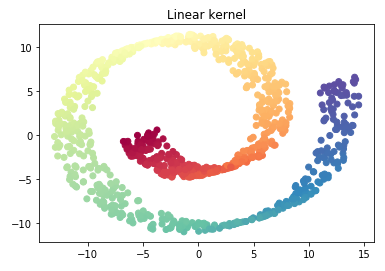

rbf_pca = KernelPCA(n_components = 2, kernel='rbf', gamma=0.04)

rbf_pca.fit(swiss_roll)

X_reduced_rbf = rbf_pca.transform(swiss_roll)

X_reduced_rbf.shape

plt.scatter(X_reduced_rbf[:, 0], X_reduced_rbf[:, 1], c = color, cmap=plt.cm.Spectral)
plt.title("RBF kernel, gamma: 0.04")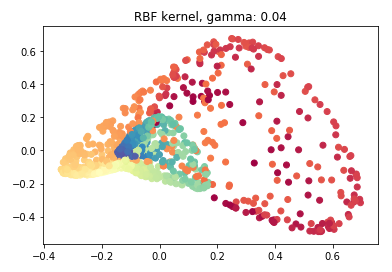

sigmoid_pca = KernelPCA(n_components = 2, kernel='sigmoid', gamma=0.001)

sigmoid_pca.fit(swiss_roll)

X_reduced_sigmoid = sigmoid_pca.transform(swiss_roll)

X_reduced_sigmoid.shape

plt.scatter(X_reduced_sigmoid[:, 0], X_reduced_sigmoid[:, 1], c = color, cmap=plt.cm.Spectral)
plt.title("RBF kernel, gamma: 0.04")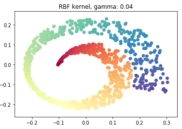

8 Tuning Hyperparameters

For this chapter let’s create some new test data:

Xmoon, ymoon = make_moons(500, noise=.06)
plt.scatter(Xmoon[:, 0], Xmoon[:, 1])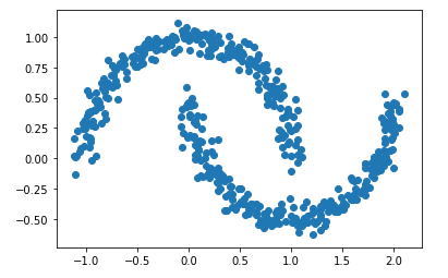

If we use a kernel PCA as a preprocessing step in order to train a machine learning algorithm, the most suitable kernel can also be calculated with the help of gridsearch.

x = Xmoon
y = ymoon

trainX, testX, trainY, testY = train_test_split(x, y, test_size = 0.2)

clf = Pipeline([
    ("kpca", KernelPCA(n_components=2)),
    ("log_reg", LogisticRegression())
    ])

param_grid = [{
    "kpca__gamma": np.linspace(0.03, 0.05, 10),
    "kpca__kernel": ["linear", "rbf", "sigmoid"]
    }]

grid_search = GridSearchCV(clf, param_grid, cv=3)

grid_search.fit(trainX, trainY)

Here are the best parameters to use:

print(grid_search.best_params_)

9 Conclusion

In this post I have explained what the PCA is in general and how to use it. I also presented different types of PCAs for different situations.

Principal Component Analysis (PCA)