1 Introduction

There are automated machine learning libraries not only for classification or regression but also for time series prediction.

This is the topic of this post.

In this post I will introduce two packages that I find quite useful to find out which algorithm fits for my time series:

Where the latter has less to do with automated machine learning but is fast and easy to use in terms of multiple models and ensembles.

2 Import the Libraries and the Functions

import pandas as pd
import numpy as np

import matplotlib.pyplot as plt
from sklearn import metrics

from statsmodels.tsa.stattools import adfuller
import ast

import warnings
warnings.filterwarnings("ignore")


# Libraries for AutoTS
from autots import AutoTS
from autots import model_forecast


# Libraries for Merlion
from merlion.utils import TimeSeries
from merlion.models.defaults import DefaultForecasterConfig, DefaultForecaster

from merlion.models.forecast.arima import Arima, ArimaConfig
from merlion.models.forecast.prophet import Prophet, ProphetConfig
from merlion.models.forecast.smoother import MSES, MSESConfig

from merlion.transform.base import Identity
from merlion.transform.resample import TemporalResample

from merlion.evaluate.forecast import ForecastMetric
from merlion.models.ensemble.combine import Mean, ModelSelector
from merlion.models.ensemble.forecast import ForecasterEnsemble, ForecasterEnsembleConfig

def mean_absolute_percentage_error_func(y_true, y_pred):
    '''
    Calculate the mean absolute percentage error as a metric for evaluation
    
    Args:
        y_true (float64): Y values for the dependent variable (test part), numpy array of floats 
        y_pred (float64): Predicted values for the dependen variable (test parrt), numpy array of floats
    
    Returns:
        Mean absolute percentage error 
    '''    
    y_true, y_pred = np.array(y_true), np.array(y_pred)
    return np.mean(np.abs((y_true - y_pred) / y_true)) * 100

def timeseries_evaluation_metrics_func(y_true, y_pred):
    '''
    Calculate the following evaluation metrics:
        - MSE
        - MAE
        - RMSE
        - MAPE
        - R²
    
    Args:
        y_true (float64): Y values for the dependent variable (test part), numpy array of floats 
        y_pred (float64): Predicted values for the dependen variable (test parrt), numpy array of floats
    
    Returns:
        MSE, MAE, RMSE, MAPE and R² 
    '''    
    print('Evaluation metric results: ')
    print(f'MSE is : {metrics.mean_squared_error(y_true, y_pred)}')
    print(f'MAE is : {metrics.mean_absolute_error(y_true, y_pred)}')
    print(f'RMSE is : {np.sqrt(metrics.mean_squared_error(y_true, y_pred))}')
    print(f'MAPE is : {mean_absolute_percentage_error_func(y_true, y_pred)}')
    print(f'R2 is : {metrics.r2_score(y_true, y_pred)}',end='\n\n')

def Augmented_Dickey_Fuller_Test_func(timeseries , column_name):
    '''
    Calculates statistical values whether the available data are stationary or not 
    
    Args:
        series (float64): Values of the column for which stationarity is to be checked, numpy array of floats 
        column_name (str): Name of the column for which stationarity is to be checked
    
    Returns:
        p-value that indicates whether the data are stationary or not
    ''' 
    print (f'Results of Dickey-Fuller Test for column: {column_name}')
    adfTest = adfuller(timeseries, autolag='AIC')
    dfResults = pd.Series(adfTest[0:4], index=['ADF Test Statistic','P-Value','# Lags Used','# Observations Used'])
    for key, value in adfTest[4].items():
       dfResults['Critical Value (%s)'%key] = value
    print (dfResults)
    if adfTest[1] <= 0.05:
        print()
        print("Conclusion:")
        print("Reject the null hypothesis")
        print('\033[92m' + "Data is stationary" + '\033[0m')
    else:
        print()
        print("Conclusion:")
        print("Fail to reject the null hypothesis")
        print('\033[91m' + "Data is non-stationary" + '\033[0m')

def inverse_diff_func(actual_df, pred_df):
    '''
    Transforms the differentiated values back
    
    Args:
        actual dataframe (float64): Values of the columns, numpy array of floats 
        predicted dataframe (float64): Values of the columns, numpy array of floats 
    
    Returns:
        Dataframe with the predicted values
    '''
    df_temp = pred_df.copy()
    columns = actual_df.columns
    for col in columns: 
        df_temp[str(col)+'_inv_diff'] = actual_df[col].iloc[-1] + df_temp[str(col)].cumsum()
    return df_temp

3 Import the Data

For this post the dataset FB from the statistic platform Kaggle was used. You can download it from my GitHub Repository.

df = pd.read_csv('FB.csv')
df = df[['Date', 'Open', 'High', 'Low', 'Close']]
df.index = pd.to_datetime(df.Date)
df = df.drop('Date', axis=1)
df.head()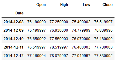

X = df[['Close']]

trainX = X.iloc[:-30]
testX = X.iloc[-30:]

4 AutoTS

With AutoTS you have the possibility to test all kinds of ML algorithms that are suitable for analyzing and predicting time series.

Here is the corresponding GitHub repository

You can find the exact documentation here: AutoTS

4.1 Compare Models

model = AutoTS(
    forecast_length=30,
    frequency='d', #for daily
    prediction_interval=0.9,
    model_list='all', 
    transformer_list='all',
    max_generations=7,
    num_validations=3,
    validation_method='similarity',
    n_jobs=-1)

For the parameter model_list there are some settings that can be made:

defined list of algorithms e.g. [‘GSL’, ‘LastValueNaive’ …]
‘superfast’
‘fast’
‘fast_parallel’
‘all’
‘default’
‘probabilistic’
‘multivariate’

For a detailed description of the parameters, please read the documentation.

model = model.fit(trainX)

Let’s display the model parameters:

best_model_Name = model.best_model_name
best_model_Parameters = model.best_model_params
best_model_TransformationParameters = model.best_model_transformation_params

print('Best model:')
print(best_model_Name)
print()
print('Model parameter of best model:')
print(best_model_Parameters)
print()
print('Transformation parameter of best model:')
print(best_model_TransformationParameters)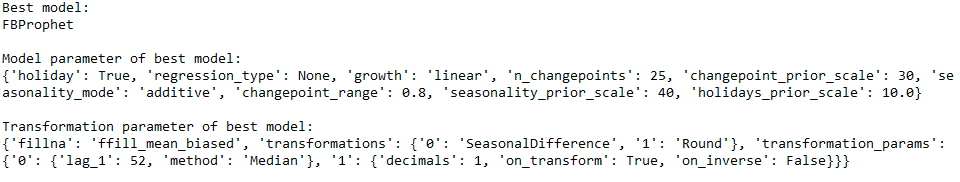

Now it is time to do the prediction and validation:

prediction = model.predict()
prediction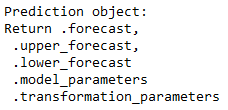

prediction.plot(model.df_wide_numeric,
                series=model.df_wide_numeric.columns[0],
                start_date="2019-01-01")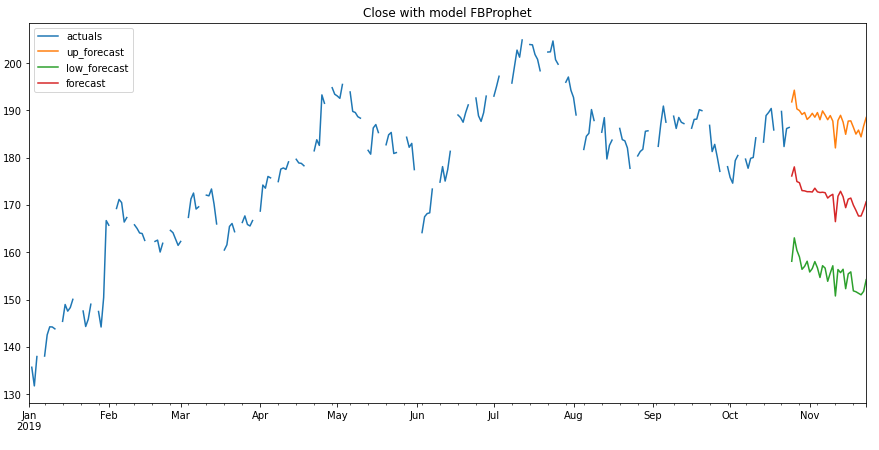

If you wonder why there are gaps in this chart, it is because the stock price is only documented from Monday to Friday. The weekend or holidays are not considered in the data set.

But that doesn’t matter, we can also display the chart again more nicely. But first let’s have a look at the validation metrics:

forecasts_df = prediction.forecast
forecasts_up, forecasts_low = prediction.upper_forecast, prediction.lower_forecast

timeseries_evaluation_metrics_func(testX, forecasts_df)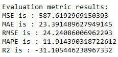

plt.rcParams["figure.figsize"] = [15,7]
plt.plot(trainX, label='Train ')
plt.plot(testX, label='Test ')
plt.plot(forecasts_df, label='Predicted ')
plt.plot(forecasts_up, label='Confidence Interval Upper bound ')
plt.plot(forecasts_low, label='Confidence Interval Lower bound ')
plt.legend(loc='best')
plt.show()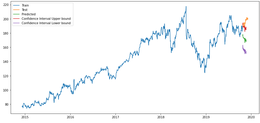

With the following command we get all calculated models including their parameters and achieved score:

model_results = model.results()
model_results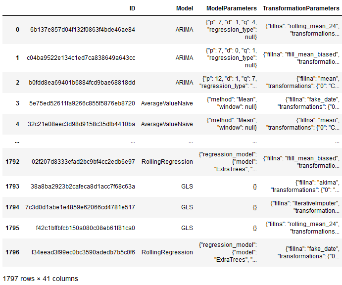

4.2 Train a single Model

Of course, you also have the possibility to train certain models specifically. Since FBProphet seems to be the best model for the data set at hand, I would like to use this algorithm specifically.

If you want to use another specific algorithm is here a list of models available in AutoTS: Models in AutoTS

Here again the parameters that led to the best result for FBProphet:

print('Best model:')
print(best_model_Name)
print()
print('Model parameter of best model:')
print(best_model_Parameters)
print()
print('Transformation parameter of best model:')
print(best_model_TransformationParameters)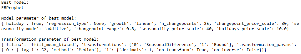

I could now enter the parameters as follows:

FBProphet_model = model_forecast(
    model_name="FBProphet",
    model_param_dict={'holiday': True, 'regression_type': None, 'growth': 'linear', 
                      'n_changepoints': 25, 'changepoint_prior_scale': 30, 
                      'seasonality_mode': 'additive', 'changepoint_range': 0.8, 
                      'seasonality_prior_scale': 40, 'holidays_prior_scale': 10.0},
    model_transform_dict={
        'fillna': 'ffill_mean_biased',
        'transformations': {'0': 'SeasonalDifference', 
                            '1': 'Round'},
        'transformation_params': {'0': {'lag_1': 52, 'method': 'Median'}, 
                                  '1': {'decimals': 1, 'on_transform': True, 'on_inverse': False}}},
    df_train=trainX,
    forecast_length=30)

But after I am too lazy to transcribe everything I can also use the saved metrics from the best model of AutoTS. I just have to format them as a dictionary.

best_model_Parameters_dic = ast.literal_eval(str(best_model_Parameters))
best_model_TransformationParameters_dic = ast.literal_eval(str(best_model_TransformationParameters))

LastValueNaive_model = model_forecast(
    model_name = best_model_Name,
    model_param_dict = best_model_Parameters_dic,
    model_transform_dict = best_model_TransformationParameters_dic,
    df_train = trainX,
    forecast_length=30)

forecasts_df_LastValueNaive_model = LastValueNaive_model.forecast
forecasts_df_LastValueNaive_model.head()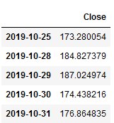

timeseries_evaluation_metrics_func(testX, forecasts_df_LastValueNaive_model)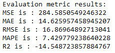

OK why is this result now again better than the one achieved before with FBProphet? This has to do with the fact that we had used cross vailidation (n=3) before.

Let’s display the results:

plt.rcParams["figure.figsize"] = [15,7]
plt.plot(trainX, label='Train ')
plt.plot(testX, label='Test ')
plt.plot(forecasts_df_LastValueNaive_model, label='Predicted ')
plt.legend(loc='best')
plt.show()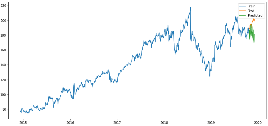

Looks better already.

4.3 Compare Models with external variables

Now, the fact is that time series can be affected by other variables. We can also take this into account in our machine learning algorithms.

Let’s look at the following variables to finally predict ‘Close’:

df.head()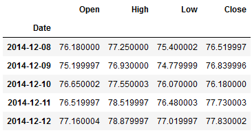

trainX_multi = df.iloc[:-30]
testX_multi = df.iloc[-30:]

We can have the values for all variables predicted with a higher weight for the target variable (‘Close’).

model_ext_var = AutoTS(
    forecast_length=30,
    frequency='d',
    prediction_interval=0.9,
    model_list='all',
    transformer_list="all",
    max_generations=7,
    num_validations=3,
    models_to_validate=0.2,
    validation_method="similarity",
    n_jobs=-1)

weights_close = {'Close': 20}

model_ext_var = model_ext_var.fit(trainX_multi,
                                  weights=weights_close)

This time it is an ensemble that gives the best result:

best_model_ext_var_Name = model_ext_var.best_model_name
best_model_ext_var_Parameters = model_ext_var.best_model_params
best_model_ext_var_TransformationParameters = model_ext_var.best_model_transformation_params

print('Best model:')
print(best_model_ext_var_Name)
print()
print('Model parameter of best model:')
print(best_model_ext_var_Parameters)
print()
print('Transformation parameter of best model:')
print(best_model_ext_var_TransformationParameters)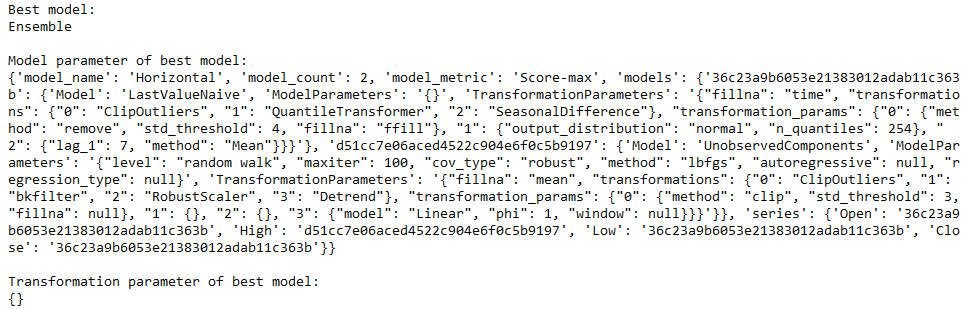

Let’s do the validation:

prediction_ext_var = model_ext_var.predict()
forecasts_df_ext_var = prediction_ext_var.forecast
forecasts_up_ext_var, forecasts_low_ext_var = prediction_ext_var.upper_forecast, prediction_ext_var.lower_forecast

for i in ['Open', 'High', 'Low', 'Close' ]:
    print(f'Evaluation metric for {i}')
    timeseries_evaluation_metrics_func(testX_multi[str(i)] , forecasts_df_ext_var[str(i)])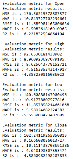

for i in ['Open', 'High', 'Low', 'Close' ]:
    
    plt.rcParams["figure.figsize"] = [10,7]
    plt.plot(trainX_multi[str(i)], label='Train '+str(i))
    plt.plot(testX_multi[str(i)], label='Test '+str(i))
    plt.plot(forecasts_df_ext_var[str(i)], label='Predicted '+str(i))
    plt.legend(loc='best')
    plt.show()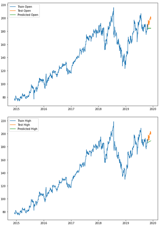

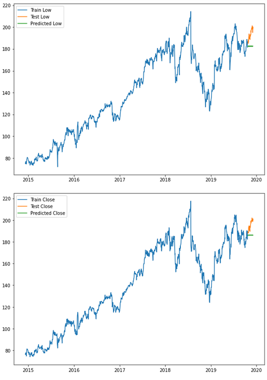
As you can see, with AutoTS you can quickly and easily get a first insight into which algorithm fits best to the dataset at hand.

5 Merlion

As mentioned at the beginning, I find Merlion quite handy for specifically testing promising algorithms for their performance to see if they fit our time series.

5.1 Prepare the Data

df.head()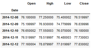

Augmented_Dickey_Fuller_Test_func(df['Close' ],'Close')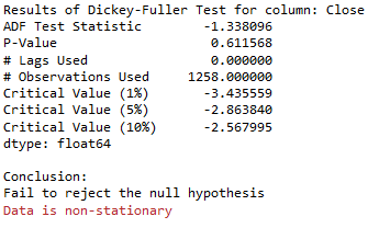

train_diff = trainX.diff()
train_diff.dropna(inplace = True)

Augmented_Dickey_Fuller_Test_func(train_diff['Close' ],'Close')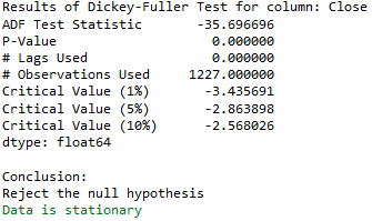

This time we differentiate our time series:

train_data = TimeSeries.from_pd(train_diff)
test_data = TimeSeries.from_pd(testX)

5.2 Default Forecaster Model

merlion_default_model = DefaultForecaster(DefaultForecasterConfig())
merlion_default_model.train(train_data=train_data)
forecast_default_model, test_err = merlion_default_model.forecast(time_stamps=test_data.time_stamps)

Admittedly, the output of the forecast is not as easy to continue using as I would like. However, we can easily transform it into a usable format:

forecast_default_model_df = pd.DataFrame(forecast_default_model).reset_index()
forecast_default_model_df.columns = ['index', 'ts', 'Value']
forecast_default_model_df['Value'] = forecast_default_model_df['Value'].astype(str)
forecast_default_model_df['Value'] = forecast_default_model_df['Value'].str.replace(',', '')
forecast_default_model_df['Value'] = forecast_default_model_df['Value'].str.replace('(', '')
forecast_default_model_df['Value'] = forecast_default_model_df['Value'].str.replace(')', '')
forecast_default_model_df['Value'] = forecast_default_model_df['Value'].astype(float)

# Assign correct index to dataframe
forecast_default_model_df = forecast_default_model_df.drop(['ts','index'], axis=1)
forecast_default_model_df.index = testX.index

# Rename the column accordingly
forecast_default_model_df.columns = ['Close']


forecast_default_model_df.head()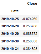

Now let’s do the inverse transformation so that the predicted values become useful.

forecast_default_model_df = inverse_diff_func(trainX, forecast_default_model_df)
forecast_default_model_df.head()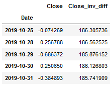

timeseries_evaluation_metrics_func(testX, forecast_default_model_df['Close_inv_diff'])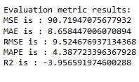

plt.rcParams["figure.figsize"] = [15,7]
plt.plot(trainX, label='Train ')
plt.plot(testX, label='Test ')
plt.plot(forecast_default_model_df['Close_inv_diff'], label='Predicted ')

plt.legend(loc='best')
plt.show()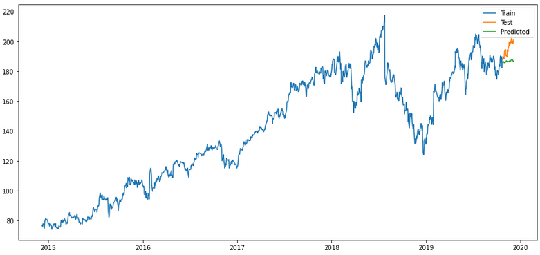

Mhhh still not the best result. Let’s see if we can improve that again.

5.3 Multiple Models & Ensembles

5.3.1 Model Config & Training

Now I am going to train multiple models as well as ensembles:

merlion_arima_model_config = ArimaConfig(max_forecast_steps=100, order=(1, 1, 1),
                                         transform=TemporalResample(granularity="D"))

merlion_arima_model  = Arima(merlion_arima_model_config)

merlion_prophet_model_config = ProphetConfig(max_forecast_steps=100, transform=Identity())

merlion_prophet_model  = Prophet(merlion_prophet_model_config)

merlion_mses_model_config = MSESConfig(max_forecast_steps=100, max_backstep=80,
                                       transform=TemporalResample(granularity="D"))

merlion_mses_model  = MSES(merlion_mses_model_config)

merlion_ensemble_model_config = ForecasterEnsembleConfig(combiner=Mean(), 
                                                         models=[merlion_arima_model, 
                                                                 merlion_prophet_model, 
                                                                 merlion_mses_model])

merlion_ensemble_model  = ForecasterEnsemble(config=merlion_ensemble_model_config)

merlion_selector_model_config = ForecasterEnsembleConfig(combiner=ModelSelector(metric=ForecastMetric.sMAPE))

merlion_selector_model = ForecasterEnsemble(config=merlion_selector_model_config, 
                                            models=[merlion_arima_model, 
                                                    merlion_prophet_model, 
                                                    merlion_mses_model])

print(f"Training {type(merlion_arima_model).__name__}:")
merlion_arima_model.train(train_data)

print(f"\nTraining {type(merlion_prophet_model).__name__}:")
merlion_prophet_model.train(train_data=train_data)

print(f"\nTraining {type(merlion_mses_model).__name__}:")
merlion_mses_model.train(train_data=train_data)

print("\nTraining ensemble model:")
merlion_ensemble_model.train(train_data=train_data)

print("\nTraining model selector:")
merlion_selector_model.train(train_data=train_data)

print()
print("Model training finished!!")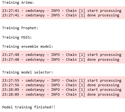

print(f"Forecasting {type(merlion_arima_model).__name__}...")
forecast_merlion_arima_model, test_err1 = merlion_arima_model.forecast(time_stamps=test_data.time_stamps)

print(f"\nForecasting {type(merlion_prophet_model).__name__}...")
forecast_merlion_prophet_model, test_err2 = merlion_prophet_model.forecast(time_stamps=test_data.time_stamps)

print(f"\nForecasting {type(merlion_mses_model).__name__}...")
forecast_merlion_mses_model, test_err3 = merlion_mses_model.forecast(time_stamps=test_data.time_stamps, 
                                                         time_series_prev=train_data)

print("\nForecasting ensemble model...")
forecast_merlion_ensemble_model, test_err_e = merlion_ensemble_model.forecast(time_stamps=test_data.time_stamps)

print("\nForecasting model selector...")
forecast_merlion_selector_model, test_err_s = merlion_selector_model.forecast(time_stamps=test_data.time_stamps, 
                                                                              time_series_prev=train_data)

print()
print()
print("Forecasting finished!!")

5.3.2 Model Evaluation

Since I don’t feel like doing the same processing steps over and over for each result, I wrote a simple function that does it for me:

def merlion_forecast_processing_func(x):
    '''
    This function is adapted to the Facebook dataframe !!  
    Brings the forecast of the Merlion models into a readable format
    
    Args:
        x (df): Y values for the dependent variable (test part), dataframe
    
    Returns:
        Processed dataframe
    '''   
    x = pd.DataFrame(x).reset_index()
    x.columns = ['index', 'ts', 'Value']
    x['Value'] = x['Value'].astype(str)
    x['Value'] = x['Value'].str.replace(',', '')
    x['Value'] = x['Value'].str.replace('(', '')
    x['Value'] = x['Value'].str.replace(')', '')
    x['Value'] = x['Value'].astype(float)
    # Assign correct index to dataframe
    x = x.drop(['ts', 'index'], axis=1)
    x.index = testX.index
    # Rename the column accordingly
    x.columns = ['Close']
    # Apply inverse_diff function
    x = inverse_diff_func(trainX, x)
    return x

forecast_merlion_arima_model_df = merlion_forecast_processing_func(forecast_merlion_arima_model)
forecast_merlion_prophet_model_df = merlion_forecast_processing_func(forecast_merlion_prophet_model)
forecast_merlion_mses_model_df = merlion_forecast_processing_func(forecast_merlion_mses_model)
forecast_merlion_ensemble_model_df = merlion_forecast_processing_func(forecast_merlion_ensemble_model)
forecast_merlion_selector_model_df = merlion_forecast_processing_func(forecast_merlion_selector_model)

merlion_arima_model

timeseries_evaluation_metrics_func(testX, forecast_merlion_arima_model_df['Close_inv_diff'])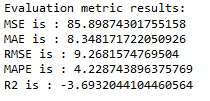

plt.rcParams["figure.figsize"] = [15,7]
plt.plot(trainX, label='Train ')
plt.plot(testX, label='Test ')
plt.plot(forecast_merlion_arima_model_df['Close_inv_diff'], label='Predicted ')

plt.legend(loc='best')
plt.show()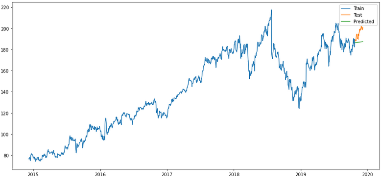

merlion_prophet_model

timeseries_evaluation_metrics_func(testX, forecast_merlion_prophet_model_df['Close_inv_diff'])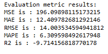

plt.rcParams["figure.figsize"] = [15,7]
plt.plot(trainX, label='Train ')
plt.plot(testX, label='Test ')
plt.plot(forecast_merlion_prophet_model_df['Close_inv_diff'], label='Predicted ')

plt.legend(loc='best')
plt.show()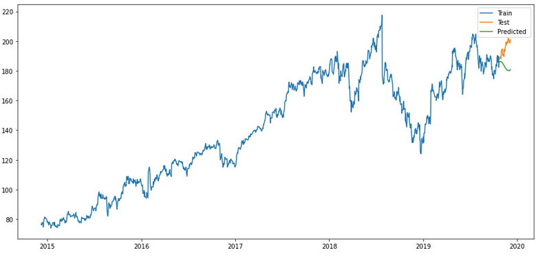

merlion_mses_model

timeseries_evaluation_metrics_func(testX, forecast_merlion_mses_model_df['Close_inv_diff'])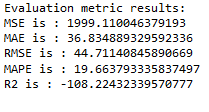

plt.rcParams["figure.figsize"] = [15,7]
plt.plot(trainX, label='Train ')
plt.plot(testX, label='Test ')
plt.plot(forecast_merlion_mses_model_df['Close_inv_diff'], label='Predicted ')

plt.legend(loc='best')
plt.show()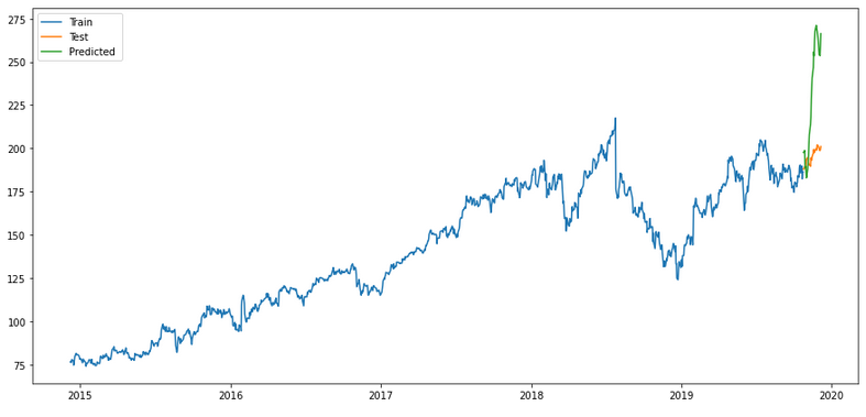

merlion_ensemble_model

timeseries_evaluation_metrics_func(testX, forecast_merlion_ensemble_model_df['Close_inv_diff'])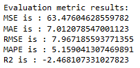

plt.rcParams["figure.figsize"] = [15,7]
plt.plot(trainX, label='Train ')
plt.plot(testX, label='Test ')
plt.plot(forecast_merlion_ensemble_model_df['Close_inv_diff'], label='Predicted ')

plt.legend(loc='best')
plt.show()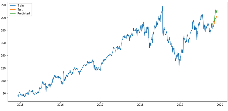

merlion_selector_model

timeseries_evaluation_metrics_func(testX, forecast_merlion_selector_model_df['Close_inv_diff'])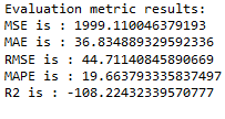

plt.rcParams["figure.figsize"] = [15,7]
plt.plot(trainX, label='Train ')
plt.plot(testX, label='Test ')
plt.plot(forecast_merlion_selector_model_df['Close_inv_diff'], label='Predicted ')

plt.legend(loc='best')
plt.show()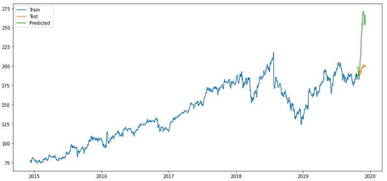

Of all the validations shown, the ensemble model seems to me to be the most promising (if only for the first half of the predictions). But ok we can either adjust that or repeat the model training after half the time.

6 Conclusion

In this post I showed how to quickly and easily figure out which algorithm(s) might fit the time series at hand to predict future values.

These are certainly not perfect yet and need to be improved but you can at least exclude some options that do not fit well and focus on the more promising algorithms.

AutoML for Time Series Analysis