1 Introduction

In my last post I introduced PyCaret and showed how to solve classification problem using this automated machine learning library. As a complement to this post, I would like to introduce the possibilities of regressions.

For this post the dataset House Sales in King County, USA from the statistic platform “Kaggle” was used. You can download it from my GitHub Repository.

2 Loading the Libraries and Data

import pandas as pd
import numpy as np

import pycaret.regression  as pycr

house_df = pd.read_csv("house_prices.csv")
house_df = house_df.drop(['zipcode', 'lat', 'long', 'date', 'id'], axis=1)
house_df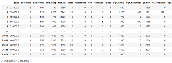

3 PyCaret - Regression

Many general options you have with PyCaret I already explained in my post about classifications. In the following I would like to go into more detail about new and regression relevant functions.

If you are not familiar with PyCaret yet, I advise you to read this post of mine first: AutoML using PyCaret - Classification

3.1 Setup

summary_preprocess = pycr.setup(house_df, 
                                target = 'price',
                                numeric_features = ['bedrooms',
                                                    'waterfront',
                                                    'view',
                                                    'condition',
                                                    'grade'],
                                normalize = True,
                                feature_interaction = True,
                                feature_ratio = True,
                                group_features = ['sqft_living', 
                                                  'sqft_lot', 
                                                  'sqft_above', 
                                                  'sqft_basement', 
                                                  'sqft_living15', 
                                                  'sqft_lot15'],
                                feature_selection = True,
                                remove_multicollinearity = True)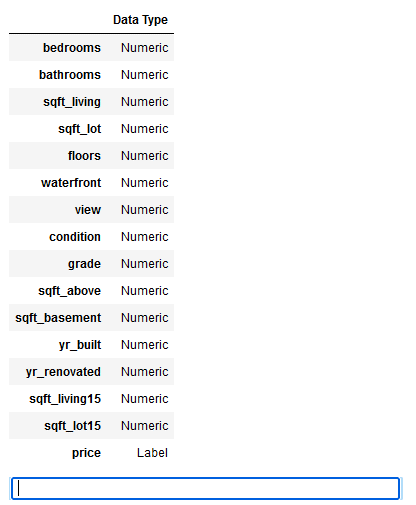

First we can check if the data types of all variables were recognized correctly. If this is the case, as here, we can press Enter.

What is different in this initiation of the setup compared to the classification post is that I have included more pre-processing steps:

Data Preparation

This time the datatype of some variables was not recognized correctly. With the parameter numeric_features=[] the correct datatype can be assigned to these variables.

Scaling

Furthermore I scaled the data this time with the normalize parameter. If you want more information about this topic see here: Feature Scaling with Scikit-Learn

Feature Engineering

Sometimes it is worthwhile to generate new features through arithmetic operations applied to existing variables. This is exactly what the feature_interaction and feature_ratio parameters do.

Here we would have two more options:

I would use these two methods if I determine that the relationship between the dependent and independent variables is not linear. Both would generate new features.

What I also did under the topic Feature Engineering is the grouping of features. This can and should be done if predictors are related in some way. Since we have different square footage data in our dataset, I want to group these features using the group_features parameter.

Feature Selection

Now that we have generated some new features by the parameters used before I would like to have it checked which of the predictors are profitable for the model training. For this I use the feature_selection.

Furthermore, I would like to counteract multicollinearity. I can do this by using the remove_multicollinearity parameter.

Important information regarding the Order of Operations!

It is important that we follow the order of operations.

In the first three steps additional features can be created whereas in the last step (feature selection) features are excluded because they violate model assumption or are not profitable for model training.

x = pycr.get_config('X')
y = pycr.get_config('y')
trainX = pycr.get_config('X_train')
testX = pycr.get_config('X_test')
trainY = pycr.get_config('y_train')
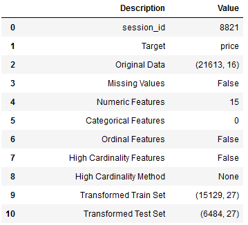
testY = pycr.get_config('y_test')

See here the number of predictors before and after pre-preocessing:

print('Number of Predictors before pre-processig: ' + str(house_df.shape[1]-1))
print('Number of Predictors after pre-processig: ' + str(x.shape[1]))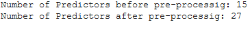

3.2 Compare Models

available_models = pycr.models()
available_models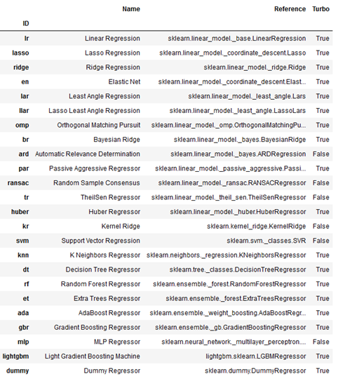

best_reg = pycr.compare_models()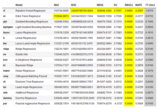

Let’s take a detailed look at the best model from the comparison:

print(best_reg)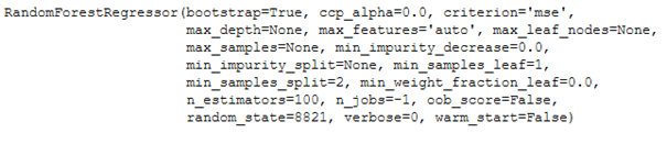

All the possible games you can do with the compare_models() function have already been described here: AutoML using PyCaret - Classification - Compare Models

3.3 Model Evaluation

evaluation_best_clf = pycr.evaluate_model(best_reg)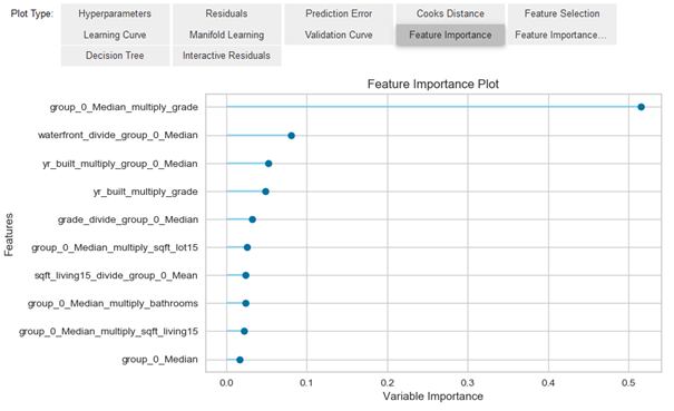

Here are a few more charts on the performance of our model:

pycr.plot_model(best_reg, plot = 'learning')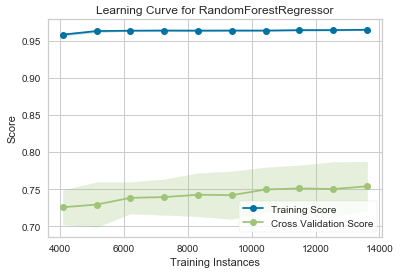

pycr.plot_model(best_reg, plot = 'error')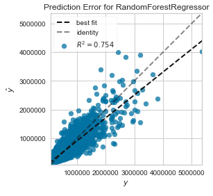

Here is an overview of possible graphics in PyCaret: Examples by module - Regression

Saving image files

If you want to save the output graphics in PyCaret, you have to set the safe parameter to True. The syntax would look like this:

pycr.plot_model(best_reg, plot = 'error',
                save = True)

3.4 Model Training

print(best_reg)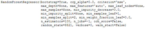

# Train the RandomForestRegressor Model 
rf_reg = pycr.create_model('rf', fold = 5)

# Obtaining the performance overview
rf_reg_results = pycr.pull()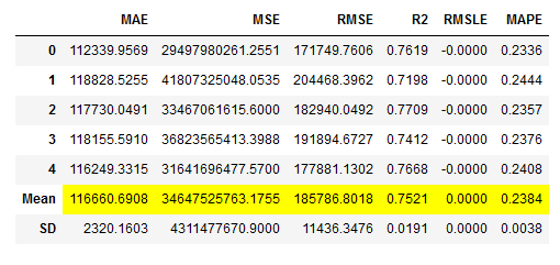

3.5 Model Optimization

In the following I will try to improve the performance of our created algorithm with different methods. At the end of the chapter I will create an overview of the performance values. On their basis I will select afterwards the final model.

3.5.1 Tune the Model

# Tune the RandomForestRegressor Model 
rf_reg_tuned, rf_reg_tuner = pycr.tune_model(rf_reg,
                                             return_tuner=True)

# Obtaining the performance overview
rf_reg_tuned_results = pycr.pull()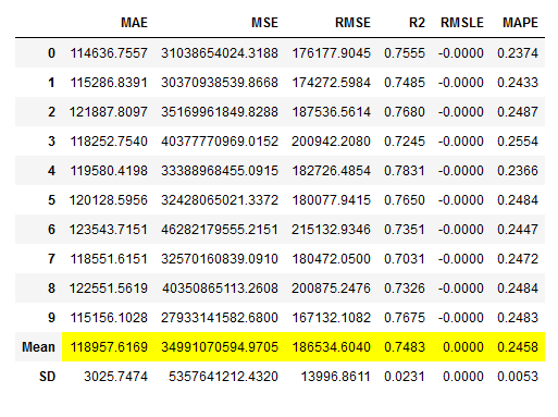

3.5.2 ensemble_models

# Train the bagged Model 
rf_reg_bagged = pycr.ensemble_model(rf_reg, 
                                    method = 'Bagging', 
                                    fold = 5,
                                    n_estimators = 30)

# Obtaining the performance overview
rf_reg_bagged_results = pycr.pull()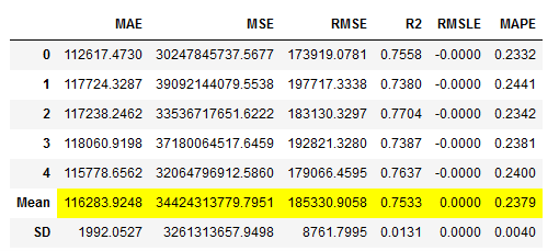

# Train the boosted Model 
rf_reg_boosted = pycr.ensemble_model(rf_reg, 
                                     method = 'Boosting', 
                                     fold = 5,
                                     n_estimators = 30)

# Obtaining the performance overview
rf_reg_boosted_results = pycr.pull()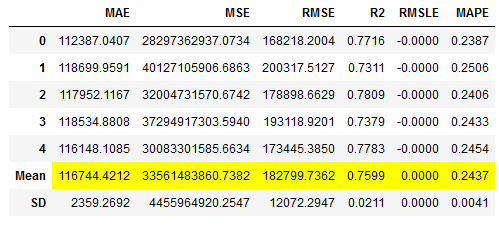

3.5.3 blend_models

Instead of selecting the models manually I will use the dynamic variant where the N best models are selected using the compare_models function and fed to the voting classifier.

# Training of N best models
voting_reg_dynamic = pycr.blend_models(pycr.compare_models(n_select = 3))

# Obtaining the performance overview
voting_reg_dynamic_results = pycr.pull()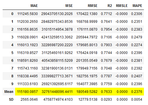

voting_reg_dynamic.estimators_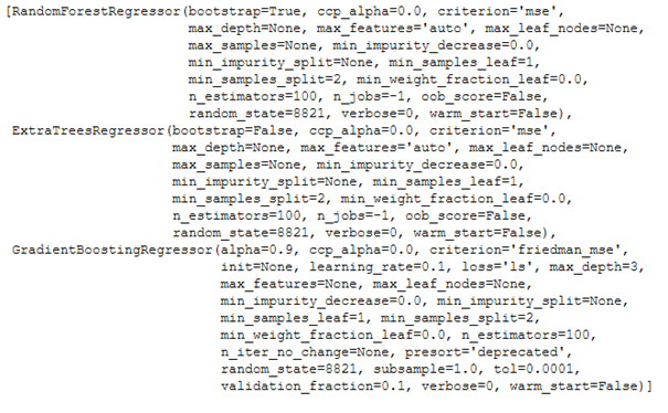

3.5.4 stack_models

# Training of N best models
stacked_reg_dynamic = pycr.stack_models(pycr.compare_models(n_select = 3))

# Obtaining the performance overview
stacked_reg_dynamic_results = pycr.pull()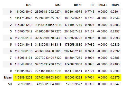

stacked_reg_dynamic.estimators_

3.5.5 Performance Overview

As announced at the beginning of this chapter, I conclude with an overview of the performance metrics that were achieved:

rf_reg_results_df = rf_reg_results.loc[['Mean']]
rf_reg_tuned_results_df = rf_reg_tuned_results.loc[['Mean']]
rf_reg_bagged_results_df = rf_reg_bagged_results.loc[['Mean']]
rf_reg_boosted_results_df = rf_reg_boosted_results.loc[['Mean']]
voting_reg_dynamic_results_df = voting_reg_dynamic_results.loc[['Mean']]
stacked_reg_dynamic_results_df = stacked_reg_dynamic_results.loc[['Mean']]


comparison_df = pd.concat([rf_reg_results_df,
                           rf_reg_tuned_results_df,
                           rf_reg_bagged_results_df,
                           rf_reg_boosted_results_df,
                           voting_reg_dynamic_results_df,
                           stacked_reg_dynamic_results_df]).reset_index()

comparison_df = comparison_df.drop('index', axis=1) 
comparison_df.insert(0, "Model", ['rf_reg', 
                                  'rf_reg_tuned', 
                                  'rf_reg_bagged',
                                  'rf_reg_boosted',
                                  'voting_reg_dynamic',
                                  'stacked_reg_dynamic'])

comparison_df.style.highlight_max(axis=0, 
                                  color = 'lightgreen', 
                                  subset=['R2']).highlight_min(axis=0, 
                                                               color = 'lightgreen', 
                                                               subset=['MAE','MSE',
                                                                       'RMSE','RMSLE','MAPE'])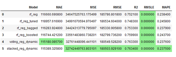

3.6 Model Evaluation after Training

type(stacked_reg_dynamic)

pycr.plot_model(stacked_reg_dynamic, plot = 'residuals')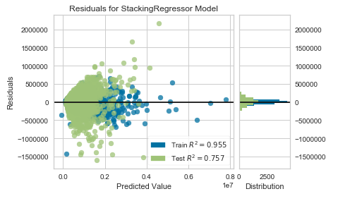

pycr.plot_model(stacked_reg_dynamic, plot = 'error')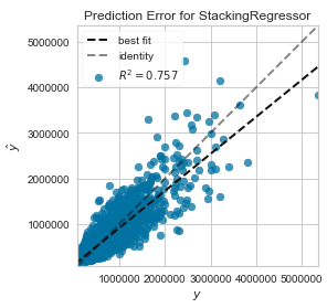

3.7 Model Predictions

# Make model predictions on testX
stacked_reg_dynamic_pred = pycr.predict_model(stacked_reg_dynamic)
stacked_reg_dynamic_pred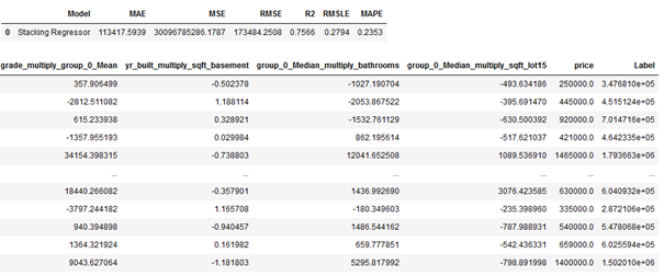

subset_stacked_reg_dynamic_pred = stacked_reg_dynamic_pred[['price', 'Label']]
subset_stacked_reg_dynamic_pred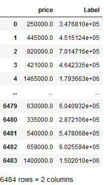

subset_stacked_reg_dynamic_pred.round(2)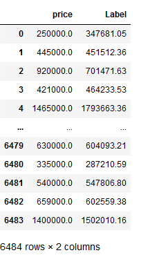

# Obtaining the performance overview
stacked_reg_dynamic_pred_results = pycr.pull()
stacked_reg_dynamic_pred_results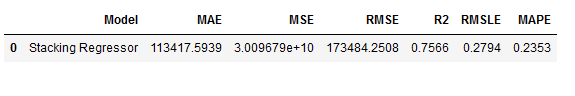

3.8 Model Finalization

stacked_reg_dynamic_final = pycr.finalize_model(stacked_reg_dynamic)
stacked_reg_dynamic_final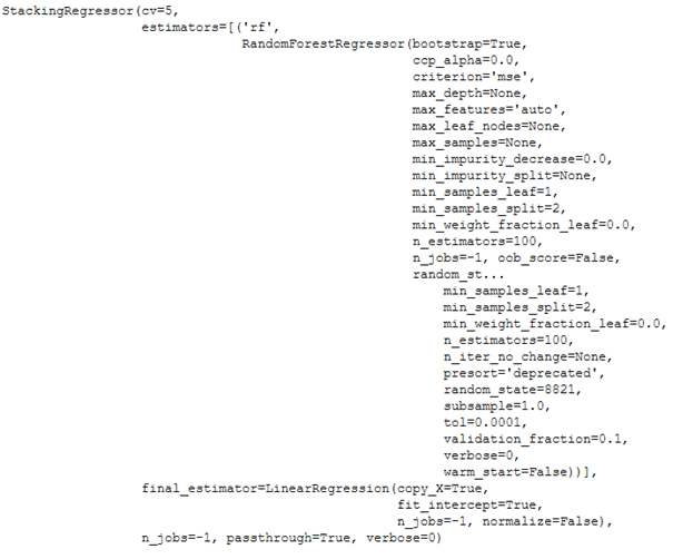

3.9 Saving the Pipeline & Model

pycr.save_model(stacked_reg_dynamic_final, 
                'stacked_reg_dynamic_final_pipeline')

Reload a Pipeline

pipeline_reload = pycr.load_model('stacked_reg_dynamic_final_pipeline')

unseen_df = pd.DataFrame(np.array([[3,2.25,1170,1249,3,0,0,3,8,1170,0,2014,0,1350,1310]]),
                          columns=['bedrooms', 'bathrooms', 'sqft_living', 'sqft_lot', 'floors', 
                                   'waterfront', 'view', 'condition', 'grade', 'sqft_above',
                                   'sqft_basement', 'yr_built', 'yr_renovated', 'sqft_living15', 'sqft_lot15'])


unseen_df

pipeline_reload_pred_unseen = pycr.predict_model(pipeline_reload,
                                                 data = unseen_df)

pipeline_reload_pred_unseen

Works !

4 Conclusion

In this post I showed how to solve regression problems using the AutoML library PyCaret. In addition to the equivalent post about classifications (AutoML using PyCaret - Classification), I went into the regression-specific functions and applications.

Limitations

I used only one version of the setup in this post. Other scaling options or feature engineering methods were not tried. Also, the handling of outliers was not considered, which could have improved the model.

AutoML using PyCaret - Regression