1 Introduction
Feature scaling can be an important part for many machine learning algorithms. It’s a step of data pre-processing which is applied to independent variables or features of data. It basically helps to normalise the data within a particular range. Sometimes, it also helps in speeding up the calculations in an algorithm.
2 Loading the libraries
import pandas as pd
import numpy as np

import matplotlib
import matplotlib.pyplot as plt
import seaborn as sns
%matplotlib inline
matplotlib.style.use('ggplot')


#For chapter 3.1
from sklearn.preprocessing import StandardScaler
#For chapter 3.2
from sklearn.preprocessing import MinMaxScaler
#For chapter 3.3
from sklearn.preprocessing import RobustScaler

#For chapter 5
import pickle as pk

#For chapter 6
from sklearn.model_selection import train_test_split


pd.set_option('float_format', '{:f}'.format)
3 Scaling methods
In the following, three of the most important scaling methods are presented:
- Standard Scaler
- Min-Max Scaler
- Robust Scaler
3.1 Standard Scaler
The Standard Scaler assumes the data is normally distributed within each feature and will scale them such that the distribution is now centred around 0, with a standard deviation of 1. If you want to know wheather your data is normal distributet have a look at this post: “Check for normal distribution”
The mean and standard deviation are calculated for the feature and then the feature is scaled based on:
np.random.seed(1)

df = pd.DataFrame({
    'Col_1': np.random.normal(0, 2, 30000),
    'Col_2': np.random.normal(5, 3, 30000),
    'Col_3': np.random.normal(-5, 5, 30000)
})

df.head()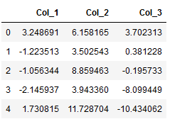
col_names = df.columns
features = df[col_names]

scaler = StandardScaler().fit(features.values)
features = scaler.transform(features.values)
scaled_features = pd.DataFrame(features, columns = col_names)
scaled_features.head()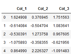
scaled_features.describe()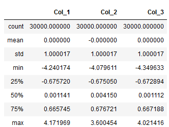
fig, (ax1, ax2) = plt.subplots(ncols=2, figsize=(6, 5))

ax1.set_title('Before Scaling')
sns.kdeplot(df['Col_1'], ax=ax1)
sns.kdeplot(df['Col_2'], ax=ax1)
sns.kdeplot(df['Col_3'], ax=ax1)
ax2.set_title('After Standard Scaler')
sns.kdeplot(scaled_features['Col_1'], ax=ax2)
sns.kdeplot(scaled_features['Col_2'], ax=ax2)
sns.kdeplot(scaled_features['Col_3'], ax=ax2)
plt.show()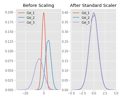
3.2 Min-Max Scaler
The Min-Max Scaler is the probably the most famous scaling algorithm, and follows the following formula for each feature:
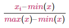
It essentially shrinks the range such that the range is now between 0 and 1. This scaler works better for cases in which the standard scaler might not work so well. If the distribution is not Gaussian or the standard deviation is very small, the Min-Max Scaler works better. However, it is sensitive to outliers, so if there are outliers in the data, you might want to consider the Robust Scaler (shown below).
np.random.seed(1)

df = pd.DataFrame({
    # positive skew
    'Col_1': np.random.chisquare(8, 1000),
    # negative skew
    'Col_2': np.random.beta(8, 2, 1000) * 40,
    # no skew
    'Col_3': np.random.normal(50, 3, 1000)
})

df.head()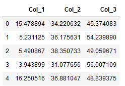
col_names = df.columns
features = df[col_names]

scaler = MinMaxScaler().fit(features.values)
features = scaler.transform(features.values)
scaled_features = pd.DataFrame(features, columns = col_names)
scaled_features.head()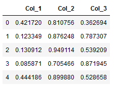
fig, (ax1, ax2) = plt.subplots(ncols=2, figsize=(6, 5))

ax1.set_title('Before Scaling')
sns.kdeplot(df['Col_1'], ax=ax1)
sns.kdeplot(df['Col_2'], ax=ax1)
sns.kdeplot(df['Col_3'], ax=ax1)
ax2.set_title('After Min-Max Scaling')
sns.kdeplot(scaled_features['Col_1'], ax=ax2)
sns.kdeplot(scaled_features['Col_2'], ax=ax2)
sns.kdeplot(scaled_features['Col_3'], ax=ax2)
plt.show()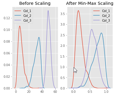
3.3 Robust Scaler
The RobustScaler uses a similar method to the Min-Max Scaler, but it instead uses the interquartile range, rathar than the Min-Max, so that it is robust to outliers. Therefore it follows the formula:
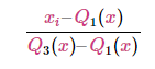
Of course this means it is using the less of the data for scaling so it’s more suitable for when there are outliers in the data.
np.random.seed(1)

df = pd.DataFrame({
    # Distribution with lower outliers
    'Col_1': np.concatenate([np.random.normal(20, 1, 1000), np.random.normal(1, 1, 25)]),
    # Distribution with higher outliers
    'Col_2': np.concatenate([np.random.normal(30, 1, 1000), np.random.normal(50, 1, 25)]),
})

df.head()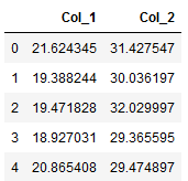
col_names = df.columns
features = df[col_names]

scaler = RobustScaler().fit(features.values)
features = scaler.transform(features.values)
scaled_features = pd.DataFrame(features, columns = col_names)
scaled_features.head()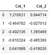
fig, (ax1, ax2) = plt.subplots(ncols=2, figsize=(6, 5))

ax1.set_title('Before Scaling')
sns.kdeplot(df['Col_1'], ax=ax1)
sns.kdeplot(df['Col_2'], ax=ax1)

ax2.set_title('After Robust Scaling')
sns.kdeplot(scaled_features['Col_1'], ax=ax2)
sns.kdeplot(scaled_features['Col_2'], ax=ax2)

plt.show()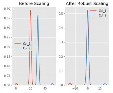
3.4 Comparison of the previously shown scaling methods
np.random.seed(32)

df = pd.DataFrame({
    # Distribution with lower outliers
    'Col_1': np.concatenate([np.random.normal(20, 1, 1000), np.random.normal(1, 1, 25)]),
    # Distribution with higher outliers
    'Col_2': np.concatenate([np.random.normal(30, 1, 1000), np.random.normal(50, 1, 25)]),
})

df.head()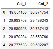
col_names = df.columns
features = df[col_names]
scaler = StandardScaler().fit(features.values)
features = scaler.transform(features.values)
standard_scaler = pd.DataFrame(features, columns = col_names)


col_names = df.columns
features = df[col_names]
scaler = MinMaxScaler().fit(features.values)
features = scaler.transform(features.values)
min_max_scaler = pd.DataFrame(features, columns = col_names)


col_names = df.columns
features = df[col_names]
scaler = RobustScaler().fit(features.values)
features = scaler.transform(features.values)
robust_scaler = pd.DataFrame(features, columns = col_names)
Now the plots in comparison:
fig, (ax1, ax2, ax3, ax4) = plt.subplots(ncols=4, figsize=(15, 7))

ax1.set_title('Before Scaling')
sns.kdeplot(df['Col_1'], ax=ax1)
sns.kdeplot(df['Col_2'], ax=ax1)

ax2.set_title('After Standard Scaler')
sns.kdeplot(standard_scaler['Col_1'], ax=ax2)
sns.kdeplot(standard_scaler['Col_2'], ax=ax2)

ax3.set_title('After Min-Max Scaling')
sns.kdeplot(min_max_scaler['Col_1'], ax=ax3)
sns.kdeplot(min_max_scaler['Col_2'], ax=ax3)

ax4.set_title('After Robust Scaling')
sns.kdeplot(robust_scaler['Col_1'], ax=ax4)
sns.kdeplot(robust_scaler['Col_2'], ax=ax4)

plt.show()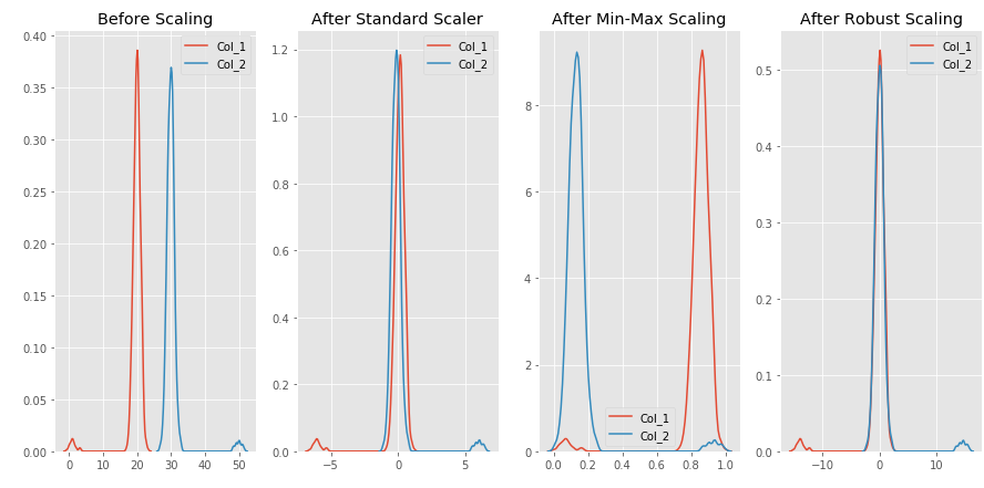
4 Inverse Transformation
As already introduced in the post about “encoders”, there is also the inverse_transform function for the scaling methods. The functionality and the procedure is very similar.
Let’s take this dataframe as an example:
df = pd.DataFrame({'Col_1': [1,7,2,4,8],
                   'Col_2': [7,1,5,3,4],
                   'Col_3': [3,8,0,3,9],
                   'Col_4': [4,7,9,1,4]})
df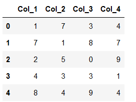
Now we apply the standard scaler as shown before:
col_names = df.columns
features = df[col_names]

scaler = StandardScaler().fit(features.values)
features = scaler.transform(features.values)
scaled_features = pd.DataFrame(features, columns = col_names)
scaled_features.head()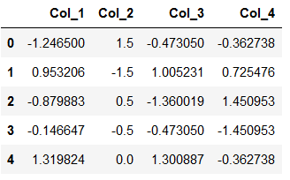
The fit scaler has memorized the metrics with which he did the transformation. Therefore it is relatively easy to do the inverse transformation with the inverse_transform function.
col_names = df.columns

re_scaled_features = scaler.inverse_transform(scaled_features)
re_scaled_df = pd.DataFrame(re_scaled_features, columns = col_names)
re_scaled_df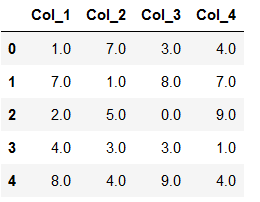
5 Export Scaler to use in another program
It is extremely important to save the used scaler separately to be able to use it again for new predictions. If you have scaled the training data with which the algorithm was created, you should also do this for predictions of new observations. In order to do this with the correct metrics, we use the originally fitted scaler.
pk.dump(scaler, open('scaler.pkl', 'wb'))
Now we reload the just saved scaler (scaler.pkl).
scaler_reload = pk.load(open("scaler.pkl",'rb'))Now we are going to use the same dataframe as bevore to see that the reloaded scaler works correctly.
df_new = pd.DataFrame({'Col_1': [1,7,2,4,8],
                   'Col_2': [7,1,5,3,4],
                   'Col_3': [3,8,0,3,9],
                   'Col_4': [4,7,9,1,4]})
df_new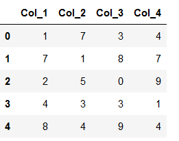
col_names2 = df_new.columns
features2 = df_new[col_names]


features2 = scaler_reload.transform(features2.values)
scaled_features2 = pd.DataFrame(features2, columns = col_names2)
scaled_features2.head()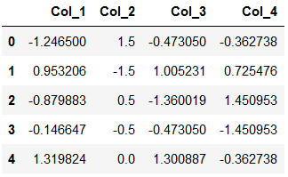
6 Feature Scaling in practice
In practice, not the complete data record is usually scaled. There are two reasons for this:
In the case of large data sets, it makes little sense with regard to the storage capacity (RAM) to reserve another scaled data set.
To train supervised machine learning algorithms, the data sets are usually divided into training and test parts. It is common to only scale the training part. The metrics used to scale the training part are then applied to the test part. This should prevent that the test part for evaluating an algorithm is really unseen.
Sounds complicated, but it’s totally easy to implement.
First of all we create a random dataframe.
df = pd.DataFrame(np.random.randint(0,100,size=(10000, 4)), columns=['Var1', 'Var2', 'Var3', 'Target_Var'])
df.head()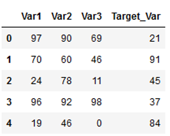
Then we split it as if we wanted to train a machine learning model. If you want to know how the train-test-split function works, have a look at this post of mine: “Random sampling”
x = df.drop('Target_Var', axis=1)
y = df['Target_Var']

trainX, testX, trainY, testY = train_test_split(x, y, test_size = 0.2)
Now the scaling is used (here StandardScaler):
sc=StandardScaler()

scaler = sc.fit(trainX)
trainX_scaled = scaler.transform(trainX)
testX_scaled = scaler.transform(testX)
We save the scaler on an object, adapt this object to the training part and transform the trainX and testX part with the metrics obtained. Here we have the scaled features:
trainX_scaled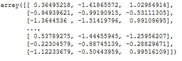
You can also save yourself a step in the syntax if you don’t use the fit & transform function individually but together!! Don’t do this if you plan to train a machine learning algorithm!! Use the previous method for this.
But if you want to scale an entire data set (for example for cluster analysis), then use the fit_transform function:
sc=StandardScaler()

df_scaled = sc.fit_transform(df)
7 Normalize or Standardize?
Scaling methods can be divided into two categories: Normalization and Standardization
As a refresher, normalization is a scaling technique where values are shifted and rescaled so that they are in the range between 0 and 1 whereas standardization centers the values around the mean with a unit standard deviation. This means that the mean value of the attribute becomes zero and the resulting distribution has a unit standard deviation.
Accordingly, the scaling methods presented above can be classified as follows:
- Standardization: Standard Scaler
- Normalization: Min-Max Scaler & Robust Scaler
The question now is when do I have to use which scaling technique? There is no single answer to this, but one can use the underlying distribution as a guide:
- Normalization is good to use when you know that the distribution of your data does not follow a Gaussian distribution.
- Standardization, on the other hand, can be helpful in cases where the data follows a Gaussian distribution.
My personal recommendation when developing machine learning models is to first fit the model to raw, normalized and standardized data and compare performance for best results.
8 Conclusion
As described in the introduction, scaling can significantly improve model performance. From this point of view, you should take these into account before training your machine learning algorithm.