1 Introduction
After I already got into the topic of Deep Learning (Computer Vision) with my past posts from January I would like to write about Neural Networks here with a more general post.
When one thinks of Deep Learning, the well-known libraries such as Keras, PyTorch or TensorFlow immediately come to mind. Most of us may not know that the very popular machine learning library Scikit-Learn is also capable of basic deep learning modeling.
How to create a neural net with this library for classification I want to show in this post.
For this publication the datasets Winequality and Iris from the statistic platform “Kaggle” were used. You can download it from my “GitHub Repository”.
2 Loading the libraries
import pandas as pd

import matplotlib.pyplot as plt

from sklearn.model_selection import train_test_split
from sklearn.preprocessing import StandardScaler


from sklearn.neural_network import MLPClassifier

from sklearn.metrics import accuracy_score
from sklearn.metrics import plot_confusion_matrix
from sklearn.metrics import classification_report

from sklearn.model_selection import GridSearchCV
3 MLPClassifier for binary Classification
The multilayer perceptron (MLP) is a feedforward artificial neural network model that maps input data sets to a set of appropriate outputs. An MLP consists of multiple layers and each layer is fully connected to the following one. The nodes of the layers are neurons with nonlinear activation functions, except for the nodes of the input layer. Between the input and the output layer there may be one or more nonlinear hidden layers.
3.1 Loading the data
df = pd.read_csv('winequality.csv').dropna()
df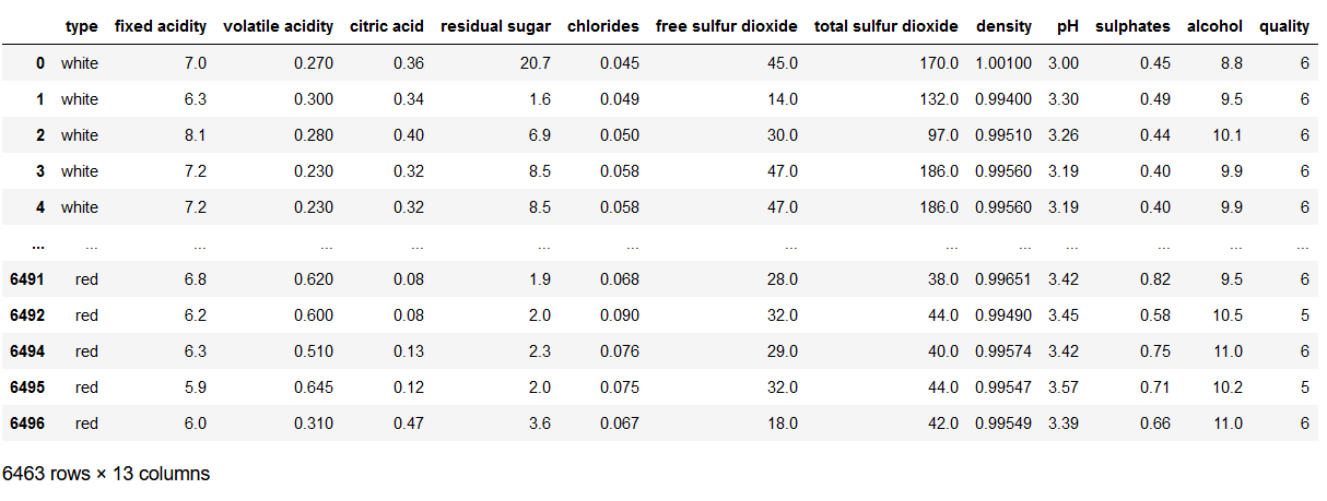
Let’s have a look at the target variable:
df['type'].value_counts()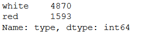
3.2 Data pre-processing
x = df.drop('type', axis=1)
y = df['type']

trainX, testX, trainY, testY = train_test_split(x, y, test_size = 0.2)
To train a MLP network, the data should always be scaled because it is very sensitive to it.
sc=StandardScaler()

scaler = sc.fit(trainX)
trainX_scaled = scaler.transform(trainX)
testX_scaled = scaler.transform(testX)
3.3 MLPClassifier
Before we train a first MLP, I’ll briefly explain something about the parameters.
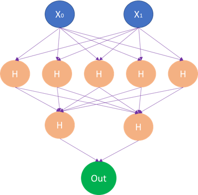
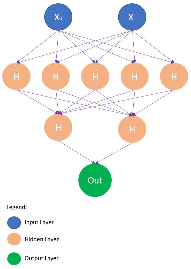
Suppose we have two predictor variables and want to do a binary classification. For this I can enter the following parameters at the model:
mlp_clf = MLPClassifier(hidden_layer_sizes=(5,2),
                        max_iter = 300,activation = 'relu',
solver = 'adam')- hidden_layer_sizes : With this parameter we can specify the number of layers and the number of nodes we want to have in the Neural Network Classifier. Each element in the tuple represents the number of nodes at the ith position, where i is the index of the tuple. Thus, the length of the tuple indicates the total number of hidden layers in the neural network.
- max_iter: Indicates the number of epochs.
- activation: The activation function for the hidden layers.
- solver: This parameter specifies the algorithm for weight optimization over the nodes.
The network structure created in the process would look like this:
So let’s train our first MLP (with a higher number of layers):
mlp_clf = MLPClassifier(hidden_layer_sizes=(150,100,50),
                        max_iter = 300,activation = 'relu',
                        solver = 'adam')

mlp_clf.fit(trainX_scaled, trainY)
3.4 Model Evaluation
The metrics that can be used to measure the performance of classification algorithms should be known. Otherwise, you can read about them here.
y_pred = mlp_clf.predict(testX_scaled)

print('Accuracy: {:.2f}'.format(accuracy_score(testY, y_pred)))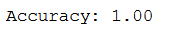
fig = plot_confusion_matrix(mlp_clf, testX_scaled, testY, display_labels=mlp_clf.classes_)
fig.figure_.suptitle("Confusion Matrix for Winequality Dataset")
plt.show()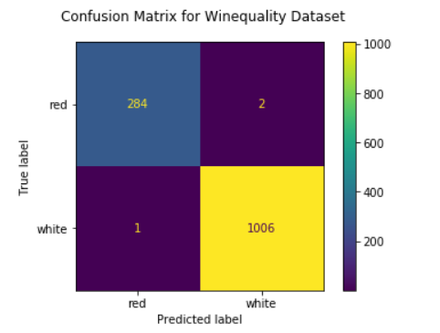
print(classification_report(testY, y_pred))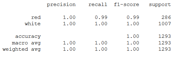
plt.plot(mlp_clf.loss_curve_)
plt.title("Loss Curve", fontsize=14)
plt.xlabel('Iterations')
plt.ylabel('Cost')
plt.show()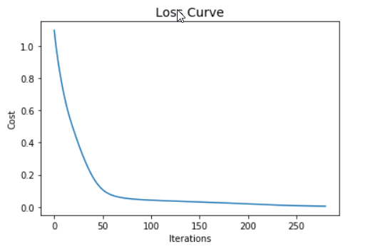
3.5 Hyper Parameter Tuning
param_grid = {
    'hidden_layer_sizes': [(150,100,50), (120,80,40), (100,50,30)],
    'max_iter': [50, 100, 150],
    'activation': ['tanh', 'relu'],
    'solver': ['sgd', 'adam'],
    'alpha': [0.0001, 0.05],
    'learning_rate': ['constant','adaptive'],
}
grid = GridSearchCV(mlp_clf, param_grid, n_jobs= -1, cv=5)
grid.fit(trainX_scaled, trainY)
print(grid.best_params_) 
grid_predictions = grid.predict(testX_scaled)

print('Accuracy: {:.2f}'.format(accuracy_score(testY, grid_predictions)))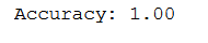
4 MLPClassifier for Multi-Class Classification
With an MLP, multi-class classifications can of course also be carried out.
4.1 Loading the data
df = pd.read_csv('Iris_Data.csv')
df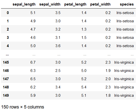
df['species'].value_counts()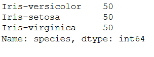
4.2 Data pre-processing
x = df.drop('species', axis=1)
y = df['species']

trainX, testX, trainY, testY = train_test_split(x, y, test_size = 0.2)
sc=StandardScaler()
scaler = sc.fit(trainX)
trainX_scaled = scaler.transform(trainX)
testX_scaled = scaler.transform(testX)4.3 MLPClassifier
mlp_clf = MLPClassifier(hidden_layer_sizes=(150,100,50),
                        max_iter = 300,activation = 'relu',
                        solver = 'adam')

mlp_clf.fit(trainX_scaled, trainY)
4.4 Model Evaluation
y_pred = mlp_clf.predict(testX_scaled)

print('Accuracy: {:.2f}'.format(accuracy_score(testY, y_pred)))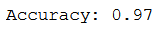
fig = plot_confusion_matrix(mlp_clf, testX_scaled, testY, display_labels=mlp_clf.classes_)
fig.figure_.suptitle("Confusion Matrix for Iris Dataset")
plt.show()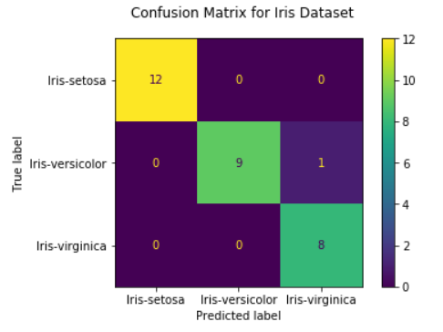
print(classification_report(testY, y_pred))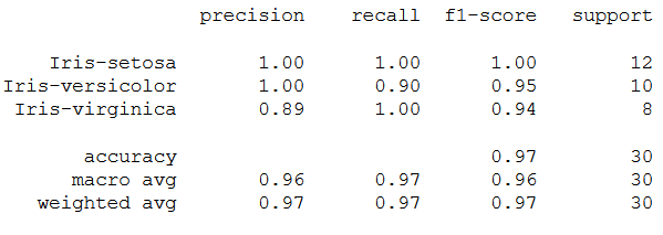
plt.plot(mlp_clf.loss_curve_)
plt.title("Loss Curve", fontsize=14)
plt.xlabel('Iterations')
plt.ylabel('Cost')
plt.show()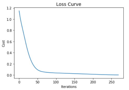
4.5 Hyper Parameter Tuning
param_grid = {
    'hidden_layer_sizes': [(150,100,50), (120,80,40), (100,50,30)],
    'max_iter': [50, 100, 150],
    'activation': ['tanh', 'relu'],
    'solver': ['sgd', 'adam'],
    'alpha': [0.0001, 0.05],
    'learning_rate': ['constant','adaptive'],
}
grid = GridSearchCV(mlp_clf, param_grid, n_jobs= -1, cv=5)
grid.fit(trainX_scaled, trainY)
print(grid.best_params_) 
grid_predictions = grid.predict(testX_scaled)

print('Accuracy: {:.2f}'.format(accuracy_score(testY, grid_predictions)))
5 Conclusion
In this post, I showed how to build an MLP model to solve binary and multi-class classification problems.