1 Introduction

Curse of Dimensionality

The curse of dimensionality is one of the most important problems in multivariate machine learning. It appears in many different forms, but all of them have the same net form and source: the fact that points in high-dimensional space are highly sparse.

I have already described two linear dimension reduction methods:

“PCA” and
“LDA”

But how do I treat data that are of a nonlinear nature? Of course we have the option of using a “Kernel-PCA” here, but that too has its limits. For this reason we can use Manifold Learning Methods, which are to be dealt with in this article.

2 Loading the libraries

import pandas as pd
import numpy as np

from sklearn import datasets
import matplotlib.pyplot as plt
from mpl_toolkits.mplot3d import Axes3D

import time


from sklearn.manifold import LocallyLinearEmbedding
from sklearn.manifold import Isomap
from sklearn.manifold import SpectralEmbedding
from sklearn.manifold import MDS
from sklearn.manifold import TSNE

3 Manifold Learning Methods

‘High-dimensional data, meaning data that requires more than two or three dimensions to represent, can be very difficult to interpret. One approach to simplification is to assume that the available data of interest lie on an embedded non-linear manifold within the higher-dimensional space. If the manifold is of low enough dimension, the data can be visualised in the low-dimensional space.’

In the following I will introduce some methods of how this is possible. For this example I will use the following data:

n_points = 1000
X, color = datasets.make_s_curve(n_points, random_state=0)

# Create figure
fig = plt.figure(figsize=(8, 8))

# Add 3d scatter plot
ax = fig.add_subplot(projection='3d')
ax.scatter(X[:, 0], X[:, 1], X[:, 2], c=color, cmap=plt.cm.Spectral)
ax.view_init(10, -70)
plt.title("Manifold Learning with an S-Curve", fontsize=15)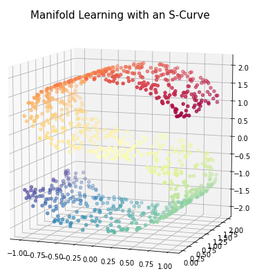

3.1 Locally Linear Embedding

Locally Linear Embedding (LLE) uses many local linear decompositions to preserve globally non-linear structures.

embedding = LocallyLinearEmbedding(n_neighbors=15, n_components=2)

X_transformed = embedding.fit_transform(X)

plt.scatter(X_transformed[:, 0], X_transformed[:, 1], c = color, cmap=plt.cm.Spectral)

plt.title('Projected data with LLE', fontsize=18)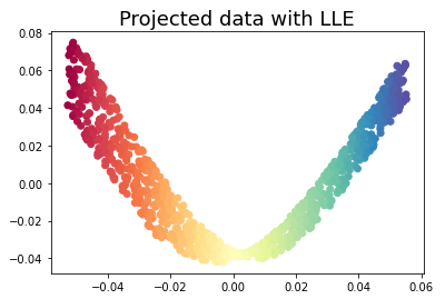

3.2 Modified Locally Linear Embedding

Modified LLE applies a regularization parameter to LLE.

embedding = LocallyLinearEmbedding(n_neighbors=15, n_components=2, method='modified')

X_transformed = embedding.fit_transform(X)

plt.scatter(X_transformed[:, 0], X_transformed[:, 1], c = color, cmap=plt.cm.Spectral)

plt.title('Projected data with modified LLE', fontsize=18)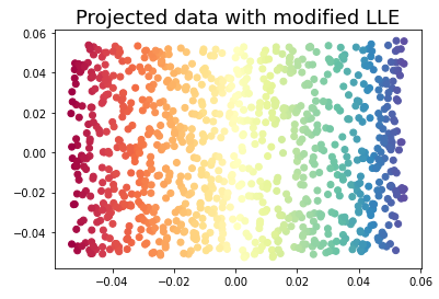

3.3 Isomap

Isomap seeks a lower dimensional embedding that maintains geometric distances between each instance.

embedding = Isomap(n_neighbors=15, n_components=2)

X_transformed = embedding.fit_transform(X)

plt.scatter(X_transformed[:, 0], X_transformed[:, 1], c = color, cmap=plt.cm.Spectral)

plt.title('Projected data with Isomap', fontsize=18)

3.4 Spectral Embedding

Spectral Embedding a discrete approximation of the low dimensional manifold using a graph representation.

embedding = SpectralEmbedding(n_neighbors=15, n_components=2)

X_transformed = embedding.fit_transform(X)

plt.scatter(X_transformed[:, 0], X_transformed[:, 1], c = color, cmap=plt.cm.Spectral)

plt.title('Projected data with Spectral Embedding', fontsize=18)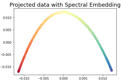

3.5 Multi-dimensional Scaling (MDS)

Multi-dimensional Scaling (MDS) uses similarity to plot points that are near to each other close in the embedding.

embedding = MDS(n_components=2)

X_transformed = embedding.fit_transform(X)

plt.scatter(X_transformed[:, 0], X_transformed[:, 1], c = color, cmap=plt.cm.Spectral)

plt.title('Projected data with MDS', fontsize=18)

3.6 t-SNE

t-SNE converts the similarity of points into probabilities then uses those probabilities to create an embedding.

embedding = TSNE(n_components=2)

X_transformed = embedding.fit_transform(X)

plt.scatter(X_transformed[:, 0], X_transformed[:, 1], c = color, cmap=plt.cm.Spectral)

plt.title('Projected data with t-SNE', fontsize=18)

4 Comparison of the calculation time

Please find below a comparison of the calculation time to the models just used.

5 Conclusion

In this post, I showed how one can graphically represent high-dimensional data using manifold learning algorithms so that valuable insights can be extracted.