1 Introduction

Now that I have written extensively about the “PCA”, we now come to another dimension reduction algorithm: The Linear Discriminant Analysis.

LDA is a supervised machine learning method that is used to separate two or more classes of objects or events. The main idea of linear discriminant analysis (LDA) is to maximize the separability between the groups so that we can make the best decision to classify them.

For this post the dataset Wine Quality from the statistic platform “Kaggle” was used. You can download it from my “GitHub Repository”.

2 Loading the libraries and data

import pandas as pd
import numpy as np

from sklearn.preprocessing import StandardScaler
from sklearn.metrics import accuracy_score
from sklearn.model_selection import train_test_split


from sklearn.decomposition import PCA

from sklearn.linear_model import LogisticRegression

from sklearn.discriminant_analysis import LinearDiscriminantAnalysis as LDA


from numpy import mean
from numpy import std

from sklearn.pipeline import Pipeline
from sklearn.model_selection import cross_val_score
from sklearn.model_selection import RepeatedStratifiedKFold
from sklearn.naive_bayes import GaussianNB
from matplotlib import pyplot

import warnings
warnings.filterwarnings('ignore')

wine = pd.read_csv('winequality.csv')
wine

3 Descriptive statistics

In the following, the variable ‘quality’ will be our target variable. Let us therefore take a look at their characteristics.

wine['quality'].value_counts()

Now let’s look at the existing data types.

wine.dtypes

Very good. All numerical variables that we need in this form in the later analysis (the variable type will be excluded). Let’s take a look at the mean values per quality class.

wine.groupby('quality').mean().T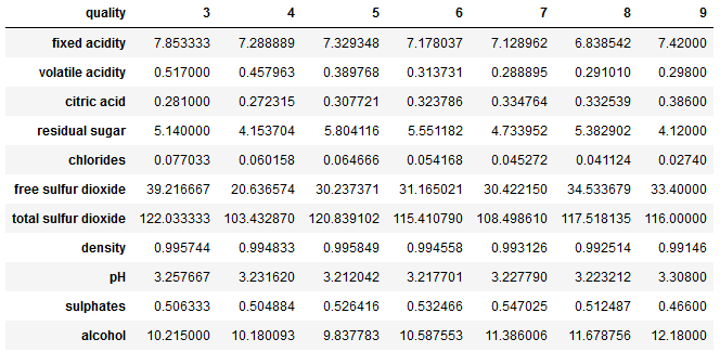

4 Data pre-processing

wine.isnull().sum()

There are a few missing values. We will now exclude these.

wine = wine.dropna()

wine.isnull().sum()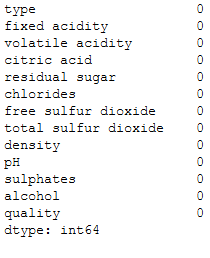

5 LDA in general

As already mentioned LDA is used to find a linear combination of features that characterizes or separates two or more classes of objects or events. It explicitly attempts to model the difference between the classes of data. It works when the measurements made on independent variables for each observation are continuous quantities. Therefore we’ll standardize our data as one of our first steps.

x = wine.drop(['type', 'quality'], axis=1)
y = wine['quality']

sc=StandardScaler()

x_scaled = sc.fit_transform(x)

lda = LDA(n_components = 2)

lda.fit(x_scaled, y)

x_lda = lda.transform(x_scaled)

As we can see from the following output we reduced the dimensions from 11 to 2.

print(x_scaled.shape)
print(x_lda.shape)

Similar to the PCA, we can have the explained variance output for these two new dimensions.

lda.explained_variance_ratio_

lda.explained_variance_ratio_.sum()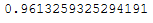

6 PCA vs. LDA

Both PCA and LDA are linear transformation techniques. However, PCA is an unsupervised while LDA is a supervised dimensionality reduction technique.

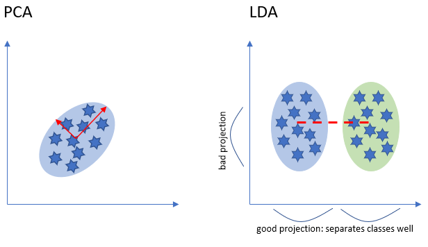
LDA is like PCA which helps in dimensionality reduction, but it focuses on maximizing the separability among known categories by creating a new linear axis and projecting the data points on that axis (see the diagram above). LDA doesn’t work on finding the principal component, it basically looks at what type of point or features gives more discrimination to separate the data.

We will use PCA and LDA when we have a linear problem in hand that means there is a linear relationship between input and output variables. When we have a nonlinear problem in hand, that means there is a nonlinear relationship between input and output variables, we will have to use the “Kernel PCA” to solve this problem.

Let’s have a look at the different results of a logistic regression when we use both, PCA and LDA, as a previous step.

x = wine.drop(['type', 'quality'], axis=1)
y = wine['quality']


trainX, testX, trainY, testY = train_test_split(x, y, test_size = 0.2)

sc=StandardScaler()

scaler = sc.fit(trainX)
trainX_scaled = scaler.transform(trainX)
testX_scaled = scaler.transform(testX)

PCA

pca = PCA(n_components = 2)

pca.fit(trainX_scaled)

pca.explained_variance_ratio_.sum()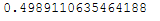

trainX_pca = pca.transform(trainX_scaled)
testX_pca = pca.transform(testX_scaled)

logReg = LogisticRegression()

logReg.fit(trainX_pca, trainY)

y_pred = logReg.predict(testX_pca)
print('Accuracy: {:.2f}'.format(accuracy_score(testY, y_pred)))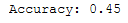

LDA

lda = LDA(n_components = 2)

lda.fit(trainX_scaled, trainY)

lda.explained_variance_ratio_.sum()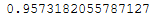

trainX_lda = lda.transform(trainX_scaled)
testX_lda = lda.transform(testX_scaled)

logReg = LogisticRegression()

logReg.fit(trainX_lda, trainY)

y_pred = logReg.predict(testX_lda)
print('Accuracy: {:.2f}'.format(accuracy_score(testY, y_pred)))

The difference in Results

The accuracy of the logistic regression model after PCA is 45% whereas the accuracy after LDA is 53%.

7 LDA as a classifier

You can also use LDA as a classifier:

lda = LDA()

lda.fit(trainX_scaled, trainY)

y_pred = lda.predict(testX_scaled)
print('Accuracy: {:.2f}'.format(accuracy_score(testY, y_pred)))

To be honest LDA is a dimensionality reduction method, not a classifier. In Scikit-Learn, the LinearDiscriminantAnalysis-class seems to be a Naive Bayes classifier after LDA “see here”.

Now that we know this, we can use the combination of LDA and Naive Bayes even more effectively.

To do this, let’s take another look at the characteristics of the target variable.

trainY.value_counts()

As we can see, we have 7 classes.

len(trainY.value_counts())

In the following, we want to build a machine learning pipeline. We want to find out with which number of components in LDA in combination with GaussianNB the prediction accuracy is greatest.

LDA is limited in the number of components used in the dimensionality reduction to between the number of classes minus one, in this case, (7 – 1) or 6. This is important for our range within the for-loop:

# get a list of models to evaluate
def get_models():
    models = dict()
    for i in range(1,7):
        steps = [('lda', LDA(n_components=i)), ('m', GaussianNB())]
        models[str(i)] = Pipeline(steps=steps)
    return models

# evaluate a give model using cross-validation
def evaluate_model(model, X, y):
    cv = RepeatedStratifiedKFold(n_splits=10, n_repeats=3, random_state=1)
    scores = cross_val_score(model, X, y, scoring='accuracy', cv=cv, n_jobs=-1, error_score='raise')
    return scores

# define dataset
X = trainX_scaled
y = trainY

# get the models to evaluate
models = get_models()

# evaluate the models and store results
results, names = list(), list()
for name, model in models.items():
    scores = evaluate_model(model, X, y)
    results.append(scores)
    names.append(name)
    print('>%s %.3f (%.3f)' % (name, mean(scores), std(scores)))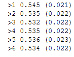

Let’s plot the results:

# plot model performance for comparison
pyplot.boxplot(results, labels=names, showmeans=True)
pyplot.show()

As we can see n_components=1 works best. So let’s use this parameter-setting to train our final model:

# define the final model
final_steps = [('lda', LDA(n_components=1)), ('m', GaussianNB())]
final_model = Pipeline(steps=final_steps)
final_model.fit(trainX_scaled, trainY)

y_pred = final_model.predict(testX_scaled)
print('Accuracy: {:.2f}'.format(accuracy_score(testY, y_pred)))

Yeah, we managed to increase the prediction accuracy again.

8 Conclusion

In this post I showed how to use the LDA and how to differentiate it from the PCA. I also showed how to use the LDA in combination with a classifier.

Linear Discriminant Analysis (LDA)