1 Introduction

As already announced in post about “PCA”, we now come to the second main application of a PCA: Principal Component Analysis for speed up machine learning models.

For this post the dataset MNIST from the statistic platform “Kaggle” was used. A copy of the record is available at https://drive.google.com/open?id=1Bfquk0uKnh6B3Yjh2N87qh0QcmLokrVk.

2 Loading the libraries and the dataset

import pandas as pd
import numpy as np

from sklearn.model_selection import train_test_split
from sklearn.preprocessing import StandardScaler
from sklearn.metrics import accuracy_score

from sklearn.linear_model import LogisticRegression

from sklearn.decomposition import PCA

import pickle as pk

mnist = pd.read_csv('mnist_train.csv')
mnist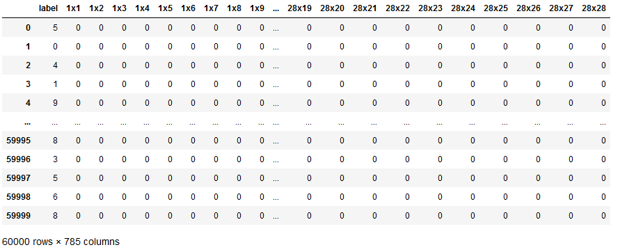

mnist['label'].value_counts().T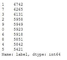

3 LogReg

If you want to know how the algorithm of the logistic regression works exactly see “this post” of mine.

x = mnist.drop(['label'], axis=1)
y = mnist['label']

trainX, testX, trainY, testY = train_test_split(x, y, test_size = 0.2)

sc=StandardScaler()

# Fit on training set only!
sc.fit(trainX)

# Apply transform to both the training set and the test set.
trainX_scaled = sc.transform(trainX)
testX_scaled = sc.transform(testX)

# all parameters not specified are set to their defaults

logReg = LogisticRegression()

import time

start = time.time()

print(logReg.fit(trainX_scaled, trainY))

end = time.time()
print()
print('Calculation time: ' + str(end - start) + ' seconds')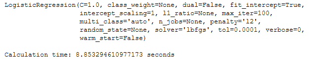

y_pred = logReg.predict(testX_scaled)

print('Accuracy: {:.2f}'.format(accuracy_score(testY, y_pred)))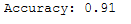

4 LogReg with PCA

4.1 PCA with 95% variance explanation

Notice the code below has .95 for the number of components parameter. It means that scikit-learn choose the minimum number of principal components such that 95% of the variance is retained.

pca = PCA(.95)

# Fitting PCA on the training set only
pca.fit(trainX_scaled)

You can find out how many components PCA choose after fitting the model using pca.n_components_ . In this case, 95% of the variance amounts to 326 principal components.

pca.n_components_

trainX_pca = pca.transform(trainX_scaled)
testX_pca = pca.transform(testX_scaled)

# all parameters not specified are set to their defaults

logReg = LogisticRegression()

import time

start = time.time()

print(logReg.fit(trainX_pca, trainY))

end = time.time()
print()
print('Calculation time: ' + str(end - start) + ' seconds')

y_pred = logReg.predict(testX_pca)

print('Accuracy: {:.2f}'.format(accuracy_score(testY, y_pred)))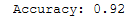

Now let’s try 80% variance explanation.

4.2 PCA with 80% variance explanation

pca = PCA(.80)

# Fitting PCA on the training set only
pca.fit(trainX_scaled)

pca.n_components_

trainX_pca = pca.transform(trainX_scaled)
testX_pca = pca.transform(testX_scaled)

# all parameters not specified are set to their defaults

logReg = LogisticRegression()

import time

start = time.time()

print(logReg.fit(trainX_pca, trainY))

end = time.time()
print()
print('Calculation time: ' + str(end - start) + ' seconds')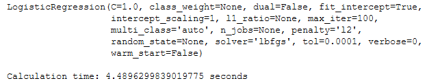

y_pred = logReg.predict(testX_pca)

print('Accuracy: {:.2f}'.format(accuracy_score(testY, y_pred)))

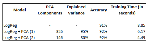
4.3 Summary

As we can see in the overview below, not only has the training time has been reduced by PCA, but the prediction accuracy of the trained model has also increased.

5 Export PCA to use in another program

For a nice example we create the following artificial data set:

df = pd.DataFrame({'Col1': [5464, 2484, 846546],
                   'Col2': [5687,78455,845684],
                   'Col3': [8754,7686,4585],
                   'Col4': [49864, 89481, 92254],
                   'Col5': [22168, 63689, 5223]})
df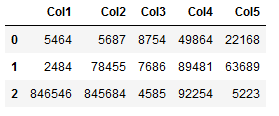

df['Target'] = df.sum(axis=1)
df

Note: We skip the scaling step and the train test split here. In the following, we only want to train the algorithms as well as their storage and use in other programs. Validation is also not a focus here.

X = df.drop(['Target'], axis=1)
Y = df['Target']

pca = PCA(n_components=2)

pca.fit(X)
result = pca.transform(X)

components = pd.DataFrame(pca.components_, columns = X.columns, index=[1, 2])
components = components.T
components.columns = ['Principle_Component_1', 'Principle_Component_2']
components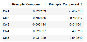

# all parameters not specified are set to their defaults

logReg = LogisticRegression()

logReg.fit(result, Y)

pk.dump(pca, open("pca.pkl","wb"))
pk.dump(logReg, open("logReg.pkl","wb"))

The models are saved in the corresponding path and should look like this:

In order to show that the principal component analysis has been saved with the correct weightings and reloaded accordingly, we create exactly the same artificial data set (only without target variable) as at the beginning of this exercise.

df_new = pd.DataFrame({'Col1': [5464, 2484, 846546],
                   'Col2': [5687,78455,845684],
                   'Col3': [8754,7686,4585],
                   'Col4': [49864, 89481, 92254],
                   'Col5': [22168, 63689, 5223]})
df_new

Now we reload the saved models:

pca_reload = pk.load(open("pca.pkl",'rb'))
logReg_reload = pk.load(open("logReg.pkl",'rb'))

result_new = pca_reload .transform(df_new)

components = pd.DataFrame(pca.components_, columns = X.columns, index=[1, 2])
components = components.T
components.columns = ['Principle_Component_1', 'Principle_Component_2']
components

We see that the weights have been adopted, as we can compare this output with the first transformation (see above).

y_pred = logReg_reload.predict(result_new)
y_pred

Last but not least we’ll add the predicted values to our original dataframe.

df_y_pred = pd.DataFrame(y_pred)
df_result_new = pd.DataFrame(result_new)

result_new = pd.concat([df_result_new, df_y_pred], axis=1)
result_new.columns = ['Principle_Component_1', 'Principle_Component_2', 'Prediction']
result_new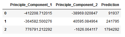

6 Conclusion

In this post, I showed how much a PCA can improve the training speed of machine learning algorithms and also increase the quality of the forecast. I also showed how the weights of principal component analysis can be saved and reused for future pre-processing steps.

PCA for speed up ML models