- 1 Introduction
- 2 Import the Libraries and the Data
- 3 Definition of required Functions
- 4 Text Pre-Processing
- 5 Conclusion
1 Introduction
Now that we have completed some pre-processing steps, I always like to start text exploration and visualization at this point.
For this publication the processed dataset Amazon Unlocked Mobile from the statistic platform “Kaggle” was used as well as the created Example String. You can download both files from my “GitHub Repository”.
2 Import the Libraries and the Data
import pandas as pd
import numpy as np

import pickle as pk

import warnings
warnings.filterwarnings("ignore")


from bs4 import BeautifulSoup
import unicodedata
import re

from nltk.tokenize import word_tokenize
from nltk.tokenize import sent_tokenize

from nltk.corpus import stopwords


from nltk.corpus import wordnet
from nltk import pos_tag
from nltk import ne_chunk

from nltk.stem.porter import PorterStemmer
from nltk.stem.wordnet import WordNetLemmatizer

from nltk.probability import FreqDist
import matplotlib.pyplot as plt
from wordcloud import WordCloud
pd.set_option('display.max_colwidth', 30)df = pd.read_csv('Amazon_Unlocked_Mobile_small_Part_IV.csv')
df.head(3).T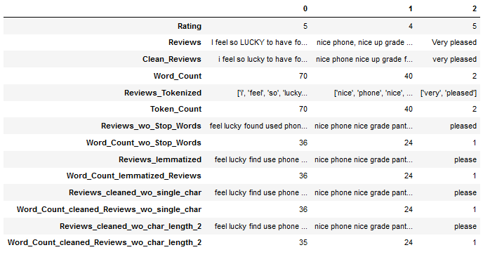
df['Reviews_cleaned_wo_single_char'] = df['Reviews_cleaned_wo_single_char'].astype(str)clean_text_wo_single_char = pk.load(open("clean_text_wo_single_char.pkl",'rb'))
clean_text_wo_single_char
3 Definition of required Functions
All functions are summarized here. I will show them again where they are used during this post if they are new and have not been explained yet.
def token_and_unique_word_count_func(text):
    '''
    Outputs the number of words and unique words

    Step 1: Use word_tokenize() to get tokens from string
    Step 2: Uses the FreqDist function to count unique words

    Args:
        text (str): String to which the functions are to be applied, string

    Prints:
        Number of existing tokens and number of unique words
    '''
    words = word_tokenize(text)
    fdist = FreqDist(words)

    print('Number of tokens: ' + str(len(words)))
    print('Number of unique words: ' + str(len(fdist)))
def most_common_word_func(text, n_words=25):
'''
Returns a DataFrame with the most commonly used words from a text with their frequencies
Step 1: Use word_tokenize() to get tokens from string
Step 2: Uses the FreqDist function to determine the word frequency
Args:
text (str): String to which the functions are to be applied, string
Returns:
A DataFrame with the most commonly occurring words (by default = 25) with their frequencies
'''
words = word_tokenize(text)
fdist = FreqDist(words)
n_words = n_words
df_fdist = pd.DataFrame({'Word': fdist.keys(),
'Frequency': fdist.values()})
df_fdist = df_fdist.sort_values(by='Frequency', ascending=False).head(n_words)
return df_fdistdef least_common_word_func(text, n_words=25):
'''
Returns a DataFrame with the least commonly used words from a text with their frequencies
Step 1: Use word_tokenize() to get tokens from string
Step 2: Uses the FreqDist function to determine the word frequency
Args:
text (str): String to which the functions are to be applied, string
Returns:
A DataFrame with the least commonly occurring words (by default = 25) with their frequencies
'''
words = word_tokenize(text)
fdist = FreqDist(words)
n_words = n_words
df_fdist = pd.DataFrame({'Word': fdist.keys(),
'Frequency': fdist.values()})
df_fdist = df_fdist.sort_values(by='Frequency', ascending=False).tail(n_words)
return df_fdist4 Text Pre-Processing
4.1 (Text Cleaning)
I have already described this part in an earlier post. See here: Text Cleaning
4.2 (Tokenization)
I have already described this part in an earlier post. See here: Text Pre-Processing II-Tokenization
4.3 (Stop Words)
I have already described this part in an earlier post. See here: Text Pre-Processing II-Stop Words
4.4 (Digression: POS & NER)
I have already described this part in an earlier post. See here: Text Pre-Processing III-POS & NER
4.5 (Normalization)
I have already described this part in an earlier post. See here: Text Pre-Processing III-Normalization
4.6 (Removing Single Characters)
I have already described this part in the previous post. See here: Text Pre-Processing IV-Removing Single Characters
4.7 Text Exploration
4.7.1 Descriptive Statistics
For better readability, I have added punctuation to the following example sentence. At this point in the text preprocessing, these would no longer be present, nor would stop words or other words with little or no information content.
But that doesn’t matter. You can use this analysis in different places, you just have to keep in mind how clean your text already is and whether punctuation marks or similar are counted.
text_for_exploration = \
"To begin to toboggan first buy a toboggan, but do not buy too big a toboggan. \
Too big a toboggan is too big a toboggan to buy to begin to toboggan."
text_for_exploration
def token_and_unique_word_count_func(text):
'''
Outputs the number of words and unique words
Step 1: Use word_tokenize() to get tokens from string
Step 2: Uses the FreqDist function to count unique words
Args:
text (str): String to which the functions are to be applied, string
Prints:
Number of existing tokens and number of unique words
'''
words = word_tokenize(text)
fdist = FreqDist(words)
print('Number of tokens: ' + str(len(words)))
print('Number of unique words: ' + str(len(fdist)))token_and_unique_word_count_func(text_for_exploration)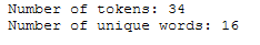
4.7.1.1 Most common Words
def most_common_word_func(text, n_words=25):
    '''
    Returns a DataFrame with the most commonly used words from a text with their frequencies

    Step 1: Use word_tokenize() to get tokens from string
    Step 2: Uses the FreqDist function to determine the word frequency

    Args:
        text (str): String to which the functions are to be applied, string

    Returns:
        A DataFrame with the most commonly occurring words (by default = 25) with their frequencies
    '''
    words = word_tokenize(text)
    fdist = FreqDist(words)

    n_words = n_words

    df_fdist = pd.DataFrame({'Word': fdist.keys(),
                             'Frequency': fdist.values()})
    df_fdist = df_fdist.sort_values(by='Frequency', ascending=False).head(n_words)

return df_fdistmost_common_word_func(text_for_exploration)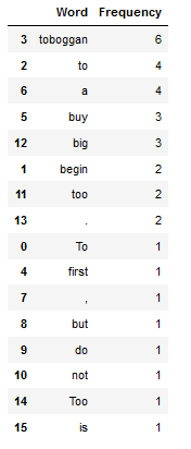
df_most_common_words_10 = most_common_word_func(text_for_exploration, n_words=10)
df_most_common_words_10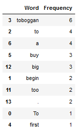
4.7.1.2 Least common Words
def least_common_word_func(text, n_words=25):
    '''
    Returns a DataFrame with the least commonly used words from a text with their frequencies

    Step 1: Use word_tokenize() to get tokens from string
    Step 2: Uses the FreqDist function to determine the word frequency

    Args:
        text (str): String to which the functions are to be applied, string

    Returns:
        A DataFrame with the least commonly occurring words (by default = 25) with their frequencies
    '''
    words = word_tokenize(text)
    fdist = FreqDist(words)

    n_words = n_words

    df_fdist = pd.DataFrame({'Word': fdist.keys(),
                             'Frequency': fdist.values()})
    df_fdist = df_fdist.sort_values(by='Frequency', ascending=False).tail(n_words)

return df_fdistleast_common_word_func(text_for_exploration, 3)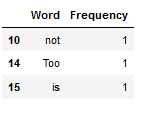
4.7.2 Text Visualization
Note: I apply the visualization only once to the most common words for now.
4.7.2.1 via Bar Charts
plt.figure(figsize=(11,7))
plt.bar(df_most_common_words_10['Word'],
        df_most_common_words_10['Frequency'])

plt.xlabel('Most common Words')
plt.ylabel("Frequency")
plt.title("Frequency distribution of the 10 most common words")

plt.show()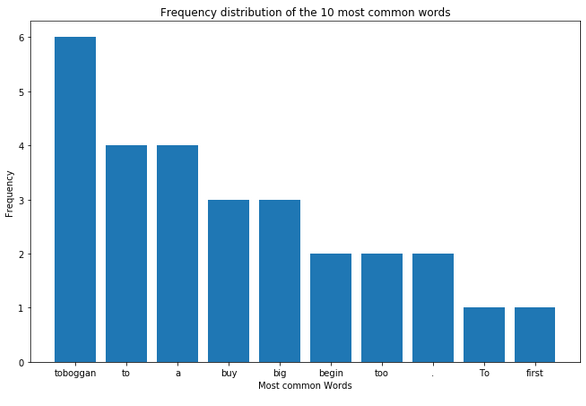
4.7.2.2 via Word Clouds
With the WordCloud function, you can also have the most frequently occurring words displayed visually. The advantage is that by default all stop words or irrelevant characters are removed from the display. The parameters that can still be set can be read here.
wordcloud = WordCloud(width = 800, height = 800,
                background_color ='white',
                min_font_size = 10).generate(text_for_exploration)

plt.figure(figsize = (8, 8), facecolor = None)
plt.imshow(wordcloud, interpolation='bilinear')
plt.axis("off")

plt.show()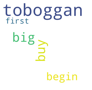
4.7.3 Application to the Example String
clean_text_wo_single_char
token_and_unique_word_count_func(clean_text_wo_single_char)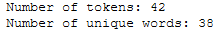
4.7.3.1 Most common Words
df_most_common_words = most_common_word_func(clean_text_wo_single_char)

df_most_common_words.head(10)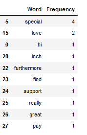
plt.figure(figsize=(11,7))
plt.bar(df_most_common_words['Word'],
        df_most_common_words['Frequency'])

plt.xticks(rotation = 45)

plt.xlabel('Most common Words')
plt.ylabel("Frequency")
plt.title("Frequency distribution of the 25 most common words")

plt.show()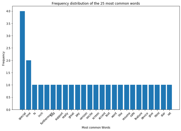
4.7.3.2 Least common Words
df_least_common_words = least_common_word_func(clean_text_wo_single_char, n_words=10)

df_least_common_words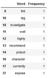
plt.figure(figsize=(11,7))
plt.bar(df_least_common_words['Word'],
        df_least_common_words['Frequency'])

plt.xticks(rotation = 45)

plt.xlabel('Least common Words')
plt.ylabel("Frequency")
plt.title("Frequency distribution of the 10 least common words")

plt.show()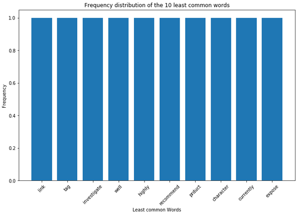
4.7.4 Application to the DataFrame
4.7.4.1 to the whole DF
As mentioned at the end of the last chapter (Removing Single Characters), I will continue to work with the ‘Reviews_cleaned_wo_single_char’ column. Here we have removed only characters with a length of 1 from the text.
In order for me to apply the functions written for this chapter, I first need to create a text corpus of all the rows from the ‘Reviews_cleaned_wo_single_char’ column.
text_corpus = df['Reviews_cleaned_wo_single_char'].str.cat(sep=' ')

text_corpus
token_and_unique_word_count_func(text_corpus)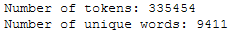
4.7.4.1.1 Most common Words
df_most_common_words_text_corpus = most_common_word_func(text_corpus)

df_most_common_words_text_corpus.head(10)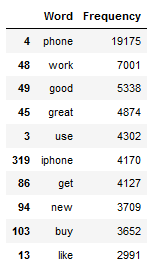
plt.figure(figsize=(11,7))
plt.bar(df_most_common_words_text_corpus['Word'],
        df_most_common_words_text_corpus['Frequency'])

plt.xticks(rotation = 45)

plt.xlabel('Most common Words')
plt.ylabel("Frequency")
plt.title("Frequency distribution of the 25 most common words")

plt.show()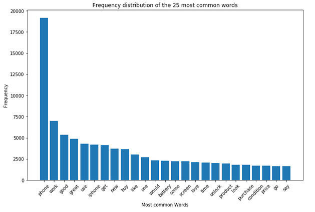
As we can see, the word ‘phone’ is by far the most common.
However, this approach is very one-sided if one considers that the comments refer to different ratings. So let’s take a closer look at them in the next step.
4.7.4.1.2 Least common Words
df_least_common_words_text_corpus = least_common_word_func(text_corpus, n_words=10)

df_least_common_words_text_corpus
plt.figure(figsize=(11,7))
plt.bar(df_least_common_words_text_corpus['Word'],
        df_least_common_words_text_corpus['Frequency'])

plt.xticks(rotation = 45)

plt.xlabel('Least common Words')
plt.ylabel("Frequency")
plt.title("Frequency distribution of the 10 least common words")

plt.show()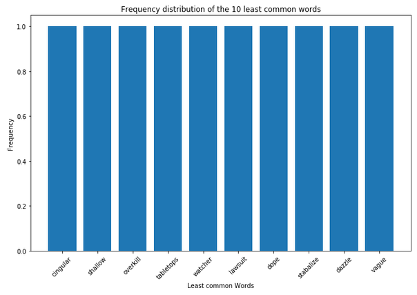
4.7.4.2 divided by Rating
As we can see from the output below, users were given the option to give 5 different ratings. The 1 stands for a bad rating and the 5 for a very good one.
df['Rating'].value_counts()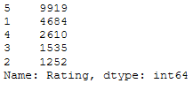
For further analysis, I will assign corresponding lables to the different ratings:
- Rating 1-2: negative
- Rating 3: neutral
- Rating 4-5: positive
I can do this using the following function:
def label_func(rating):
    if rating <= 2:
        return 'negative'
    if rating >= 4:
        return 'positive'
    else:
        return 'neutral'

df['Label'] = df['Rating'].apply(label_func)
I personally prefer to have the ‘Rating’ and ‘Label’ columns together. So far, the ‘Label’ column is at the end of the record because it was just newly created. However, the order can be changed with the following command.
Do this column reordering only once, otherwise more and more columns will be put in first place.
cols = list(df.columns)
cols = [cols[-1]] + cols[:-1]
df = df[cols]
As you can see from the partial output shown below, the labels were assigned correctly.
df.T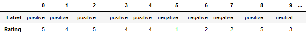
Now I divide the data set according to their labels (‘positive’, ‘neutral’ and ‘negative’).
positive_review = df[(df["Label"] == 'positive')]['Reviews_cleaned_wo_single_char']
neutral_review = df[(df["Label"] == 'neutral')]['Reviews_cleaned_wo_single_char']
negative_review = df[(df["Label"] == 'negative')]['Reviews_cleaned_wo_single_char']
According to the division, I create a separate text corpus for each.
text_corpus_positive_review = positive_review.str.cat(sep=' ')
text_corpus_neutral_review = neutral_review.str.cat(sep=' ')
text_corpus_negative_review = negative_review.str.cat(sep=' ')
Then I can use the most_common_word function again and save the results in a separate data set.
df_most_common_words_text_corpus_positive_review = most_common_word_func(text_corpus_positive_review)
df_most_common_words_text_corpus_neutral_review = most_common_word_func(text_corpus_neutral_review)
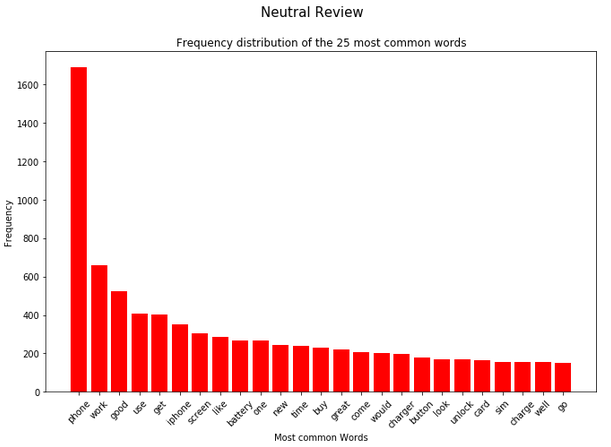
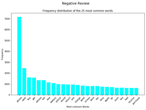
df_most_common_words_text_corpus_negative_review = most_common_word_func(text_corpus_negative_review)Now I can use a for-loop to visually display the 25 most frequently occurring words in each of the partial data sets.
splited_data = [df_most_common_words_text_corpus_positive_review,
                df_most_common_words_text_corpus_neutral_review,
                df_most_common_words_text_corpus_negative_review]

color_list = ['green', 'red', 'cyan']
title_list = ['Positive Review', 'Neutral Review', 'Negative Review']


for item in range(3):
    plt.figure(figsize=(11,7))
    plt.bar(splited_data[item]['Word'],
            splited_data[item]['Frequency'],
            color=color_list[item])
    plt.xticks(rotation = 45)
    plt.xlabel('Most common Words')
    plt.ylabel("Frequency")
    plt.title("Frequency distribution of the 25 most common words")
    plt.suptitle(title_list[item], fontsize=15)
    plt.show()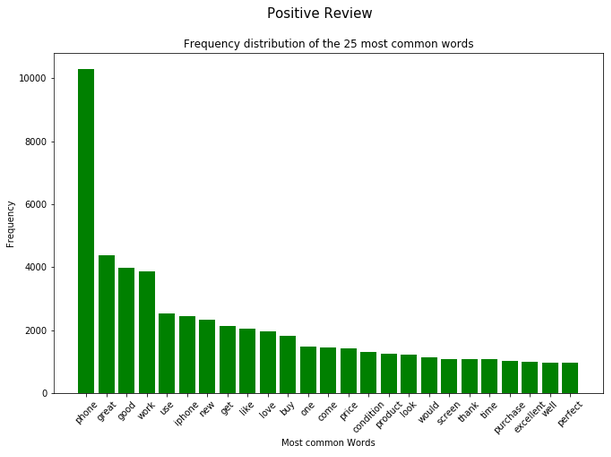
Note: I omit the same implementation for the least frequent words at this point. It would follow the same principle as I showed before.
5 Conclusion
In this post I showed how to explore and visualize text blocks easily and quickly. Based on these insights, our next steps will emerge, which I will present in the following post.
Here we only need to save the DataFrame, since we have made changes. This was not the case with the Example String.
df.to_csv('Amazon_Unlocked_Mobile_small_Part_V.csv', index = False)Furthermore, we have created some frequency tables, which we will need again in the following post. Therefore they will be saved as well.
df_most_common_words.to_csv('df_most_common_words.csv', index = False)
df_least_common_words.to_csv('df_least_common_words.csv', index = False)
df_most_common_words_text_corpus.to_csv('df_most_common_words_text_corpus.csv', index = False)
df_least_common_words_text_corpus.to_csv('df_least_common_words_text_corpus.csv', index = False)