1 Introduction

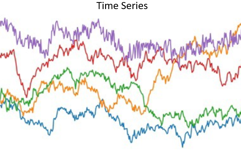
Let’s continue our journey through the different Analytics fields. Let’s now move on to the topic of Time Series Analysis. Most of the time we deal with cross-sectional data. Here, the data is collected at a specific point in time. On the other hand, time series data is a collection of observations obtained through repeated measurements over time. If we were to draw the points in a diagram then one of your axes would always be time.

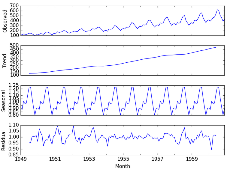
A given time series is thought to consist of four systematic components:

• Trend, which describe the movement along the term.
• Seasonality, which is the repeating short-term cycle in the series.
• Cyclic Variations, which reflects repeated but non-periodic fluctuations.
• Noise, which are random variation in the series.

We can check these, with a decomposition plot like this one shown below:

But why is this information about Time Series Components so important to us? This information influences our choice of algorithms and the pre-processing steps necessary to develop a good predictive model.

2 Import the libraries and the data

import pandas as pd
import datetime

I have created a separate dataset for this post. You can download it from my “GitHub Repository”.

df = pd.read_csv('timestamp_df.csv', usecols=['timestamp'])
df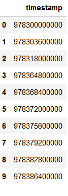

3 Convert timestamp to DateTime

# Convert timestamp to DateTime
# Admittedly in this example the timestamp is in a longer format than usual. Therefore the division by 1000

df['timestamp_epoch2'] = df.timestamp.astype(float)
df['new_timestamp_epoch'] = df.timestamp_epoch2 / 1000
df['new_timestamp_epoch_round'] = df.new_timestamp_epoch.round()
df['new_timestamp_epoch_round'] = df.new_timestamp_epoch_round.astype(int)
df['final'] = df.new_timestamp_epoch_round.map(lambda x: datetime.utcfromtimestamp(x).strftime('%Y-%m-%d %H:%M:%S'))
df['DateTime'] = pd.to_datetime(df['final'])
df.drop(["timestamp_epoch2", "new_timestamp_epoch", "new_timestamp_epoch_round", "final"], axis = 1, inplace = True) 


# Print new df
df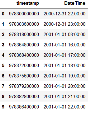

You can also use this syntax:

df['new_DateTime'] = df['new_timestamp_epoch_round'].apply(datetime.fromtimestamp)

4 Extract Year, Month and Day

df['Year'] = df.DateTime.dt.year
df['Month'] = df.DateTime.dt.month
df['Day'] = df.DateTime.dt.day

df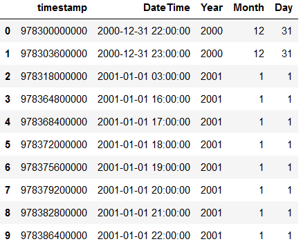

5 Extract Weekday and Week

df['Weekday'] = df.DateTime.dt.day_name()
df['Week'] = df.DateTime.dt.isocalendar().week

df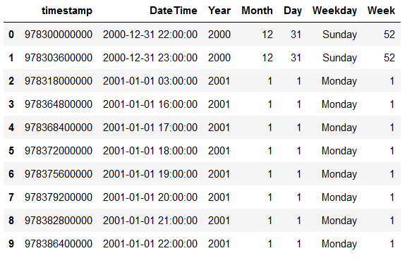

6 Calculate Quarter

For calculating the quarter I defined the following function:

def get_quarter(df):

    if (df['Month'] <= 3):
        return 'Q1'
    
    elif (df['Month'] <= 6) and (df['Month'] > 3):
        return 'Q2'
              
    elif (df['Month'] <= 9) and (df['Month'] > 6):
        return 'Q3'

    elif (df['Month'] <= 12) and (df['Month'] > 9):
        return 'Q4'

Let’s apply the defined function:

df['Quarter'] = df.apply(get_quarter, axis = 1)

df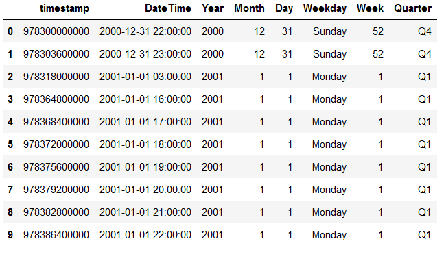

7 Generate YearQuarter

Especially for visualizations I always quite like to have the YearQuarter indication. Unfortunately, we cannot access the year with the str.-function as usual. The output would look like this:

str(df['Year'])

Let’s have a look at the column types:

df.dtypes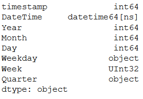

Year is here output as int64, but as we can see there is a string containing the information for all years. But we can pull the year as an object directly from DateTime.

df['DateTime'].apply(lambda x: x.strftime('%Y'))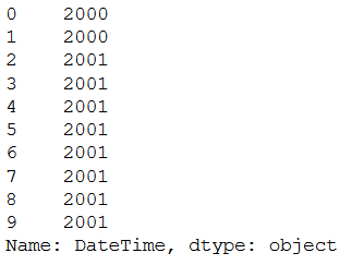

Since this solution works, we now do this to generate another column.

df['YearQuarter'] = df['DateTime'].apply(lambda x: x.strftime('%Y')) + df['Quarter']

df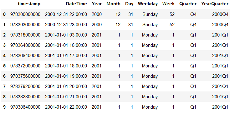

A final check:

df.dtypes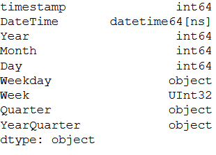

Perfect.

This also works with any other elements from DateTime. For example month or day. Here also the order can be chosen arbitrarily. Here for example: Day, month and year

df['DateTime'].apply(lambda x: x.strftime('%d%m%Y'))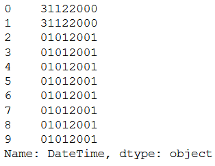

8 Filter for TimeDate

df['DateTime']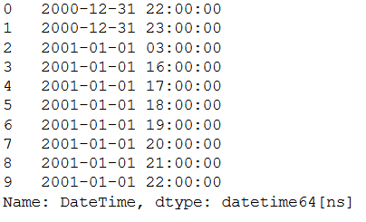

print('Oldest Date: ' + str(df['DateTime'].min()))
print('Earliest Date: ' + str(df['DateTime'].max()))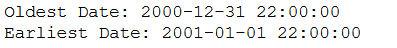

Filter by dates greater than or equal to 01.01.2001:

filter1 = df.loc[df['DateTime'] >= '2001-01-01']
filter1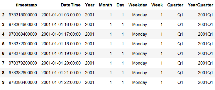

Filter by dates greater than or equal to 01.01.2001 18h00:

filter2 = df.loc[df['DateTime'] >= '2001-01-01 18']
filter2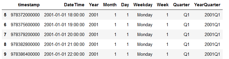

9 Conclusion

This was a smart introduction to how to handle Time Series data and how to extract more information from a Timestamp. Furthermore I went into what stationary data is and what differentiating means.