1 Introduction
2 Loading the libraries and the dataset
3 Statistics and preprocessing
4 PCA for visualization
- 4.1 Interpreting Components
- 4.2 Visualization of the components
5 Conclusion

1 Introduction

After I wrote extensively on the subject of “Principal Component Analysis” in my last publication, we now come to one of the two main uses announced: PCA for visualizations.

For this post the dataset Pokemon from the statistic platform “Kaggle” was used. You can download it from my “GitHub Repository”.

2 Loading the libraries and the dataset

import numpy as np
import pandas as pd

import math

import matplotlib.pyplot as plt
%matplotlib inline
plt.style.use('ggplot')

from sklearn.decomposition import PCA

from sklearn.preprocessing import StandardScaler

pokemon = pd.read_csv("pokemon.csv")
pokemon.head()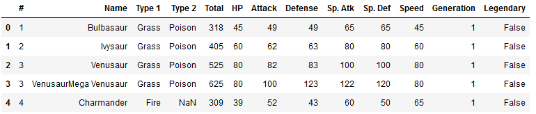

3 Statistics and preprocessing

df = pokemon[['HP', 'Attack', 'Defense', 'Sp. Atk', 'Sp. Def', 'Speed']]

df.describe()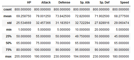

col_names = df.columns
features = df[col_names]

scaler = StandardScaler().fit(features.values)
features = scaler.transform(features.values)
df_scaled = pd.DataFrame(features, columns = col_names)
df_scaled.head()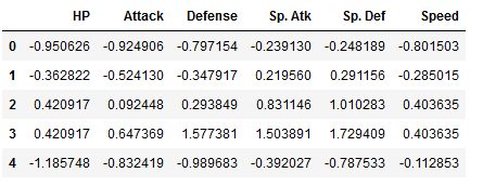

4 PCA for visualization

First of all, we calculate the first two main components using the PCA. If one of the following steps is not clear or is insufficiently described, read “this” post from me.

pca = PCA(n_components=2, svd_solver='full')

pca.fit(df_scaled)
T = pca.transform(df_scaled)

print('Here we can see that we started with 6 dimensions:')
print(df_scaled.shape)
print('')
print('After PCA we have only 2:')
print(T.shape)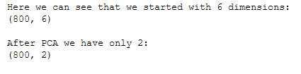

pca.explained_variance_ratio_

4.1 Interpreting Components

These are the two main components calculated:

components = pd.DataFrame(pca.components_, columns = df_scaled.columns, index=[1, 2])
components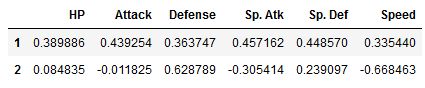

Personally, I prefer to read these in the following format:

components = components.T

components.columns = ['Principle_Component_1', 'Principle_Component_2']
components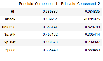

Component 1

pc1 = components[['Principle_Component_1']].sort_values(by='Principle_Component_1', ascending=False)
pc1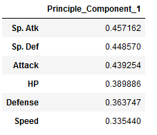

So for the first principle component, Sp. Attack and Sp. Defence is significant so this principle component is correlated well with Sp. Atk and Sp. Def and pokemon with a high value for the first principle component have high Sp. Atk and Sp. Def.

Component 2

pc2 = components[['Principle_Component_2']].sort_values(by='Principle_Component_2', ascending=False)
pc2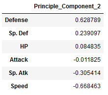

Be careful at this point. Some high values are in the minus range and are therefore only listed at the end of the table. We therefore have to convert all values into absolute values and then sort them in descending order.

pc2['positive_values'] = abs(pc2.Principle_Component_2)
pc2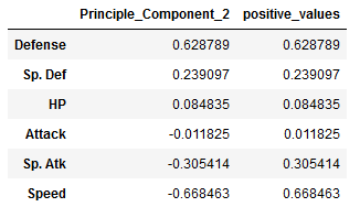

pc2.sort_values(by='positive_values', ascending=False)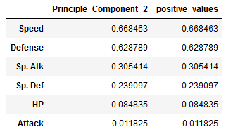

For the second principle component, this will increase with an decrease in Speed and a increase in Defence. Pokemon with high values of the second principle component will have a high value for Defense but a low value for Speed.

4.2 Visualization of the components

def get_important_features(transformed_features, components_, columns):
    """
    This function will return the most "important" 
    features so we can determine which have the most
    effect on multi-dimensional scaling
    """
    num_columns = len(columns)

    # Scale the principal components by the max value in
    # the transformed set belonging to that component
    xvector = components_[0] * max(transformed_features[:,0])
    yvector = components_[1] * max(transformed_features[:,1])

    # Sort each column by it's length. These are your *original*
    # columns, not the principal components.
    important_features = { columns[i] : math.sqrt(xvector[i]**2 + yvector[i]**2) for i in range(num_columns) }
    important_features = sorted(zip(important_features.values(), important_features.keys()), reverse=True)
    return important_features

# application of the function
important_features = get_important_features(T, pca.components_, df.columns.values)

# convert output to pd.dataframe
important_features = pd.DataFrame(important_features, columns =['Value', 'Feature'])
# change order of dataframe columns
cols = ['Feature', 'Value']
important_features = important_features[cols]

#print the output
important_features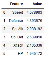

def draw_vectors(transformed_features, components_, columns):
    """
    This funtion will project your *original* features
    onto your principal component feature-space, so that you can
    visualize how "important" each one was in the
    multi-dimensional scaling
    """

    num_columns = len(columns)

    # Scale the principal components by the max value in
    # the transformed set belonging to that component
    xvector = components_[0] * max(transformed_features[:,0])
    yvector = components_[1] * max(transformed_features[:,1])

    ax = plt.axes()

    for i in range(num_columns):
    # Use an arrow to project each original feature as a
    # labeled vector on your principal component axes
        plt.arrow(0, 0, xvector[i], yvector[i], color='b', width=0.0005, head_width=0.02, alpha=0.75)
        plt.text(xvector[i]*1.2, yvector[i]*1.2, list(columns)[i], color='b', alpha=0.75)

    return ax

ax = draw_vectors(T, pca.components_, df.columns.values)
T_df = pd.DataFrame(T)
T_df.columns = ['component1', 'component2']

T_df['color'] = 'y'
T_df.loc[T_df['component1'] > 4, 'color'] = 'g'
T_df.loc[T_df['component2'] > 3, 'color'] = 'r'

plt.xlabel('Principle Component 1')
plt.ylabel('Principle Component 2')
plt.scatter(T_df['component1'], T_df['component2'], color=T_df['color'], alpha=0.5)
plt.show()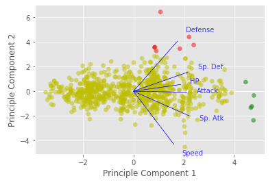

Get the pokemons which load high on the first principal component (High Sp. Atk, High Sp. Def):

pc1_pokemon = pokemon.loc[T_df[T_df['color'] == 'g'].index]
pc1_pokemon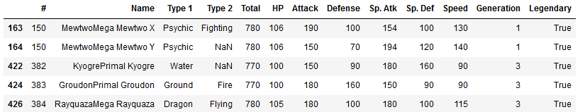

Get the pokemons which load high on the second principal component (High Defense, Low Speed):

pc2_pokemon = pokemon.loc[T_df[T_df['color'] == 'r'].index]
pc2_pokemon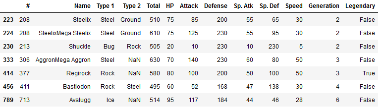

5 Conclusion

In this post, I showed how a PCA can be used sensibly to visualize complex data and extract valuable insights from it.

PCA for Visualization