1 Introduction
In my previous post “Introduction to regression analysis and predictions” I showed how to create linear regression models. But what can be done if the data is not distributed linearly?
For this post the dataset Auto-mpg from the statistic platform “Kaggle” was used. You can download it from my GitHub Repository.
2 Loading the libraries and the data
import pandas as pd
import numpy as np
import matplotlib.pyplot as plt
%matplotlib inline
import math
from sklearn.linear_model import LinearRegression
from sklearn import metrics
from sklearn.preprocessing import PolynomialFeatures
from sklearn import linear_model
cars = pd.read_csv("path/to/file/auto-mpg.csv")3 Data Preparation
cars.head()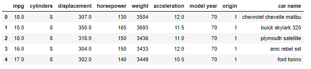
Check the data types:
cars.dtypes
Convert horsepower from an object to a float:
cars["horsepower"] = pd.to_numeric(cars.horsepower, errors='coerce')
cars.dtypes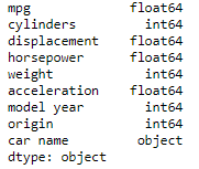
Check for missing values:
cars.isnull().sum()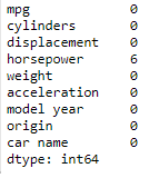
Replace the missing values with the mean of column:
cars_horsepower_mean = cars['horsepower'].fillna(cars['horsepower'].mean())
cars['horsepower'] = cars_horsepower_mean
cars.isnull().sum()    #Check replacement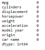
4 Hypothesis: a non-linear relationship between the variables mpg and horesepower
cars.plot(kind='scatter', x='horsepower', y='mpg', color='red')
plt.xlabel('Horsepower')
plt.ylabel('Miles per Gallon')
plt.title('Scatter Plot: Horsepower vs. Miles per Gallon')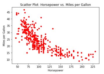
5 Linear model
First of all, the two variables ‘mpg’ and ‘horesepower’ are to be investigated with a linear regression model.
x = cars["horsepower"]
y = cars["mpg"]

lm = LinearRegression()
lm.fit(x[:,np.newaxis], y)
The linear regression model by default requires that x bean array of two dimensions. Therefore we have to use the np.newaxis-function.
cars.plot(kind='scatter', x='horsepower', y='mpg', color='red')
plt.plot(x, lm.predict(x[:,np.newaxis]), color='blue')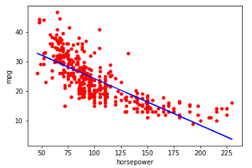
Calculation of R²
lm.score(x[:,np.newaxis], y)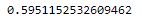
Calculation of further parameters:
y_pred = lm.predict(x[:,np.newaxis])

df = pd.DataFrame({'Actual': y, 'Predicted': y_pred})
df.head()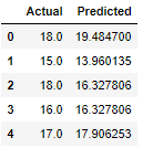
print('Mean Absolute Error:', metrics.mean_absolute_error(y, y_pred))
print('Mean Squared Error:', metrics.mean_squared_error(y, y_pred))
print('Root Mean Squared Error:', np.sqrt(metrics.mean_squared_error(y, y_pred)))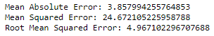
6 Non linear models
6.1 Quadratic Function
We now try using different methods of transformation, applied to the predictor, to improve the model results.
x = cars["horsepower"] * cars["horsepower"]
y = cars["mpg"]

lm = LinearRegression()
lm.fit(x[:,np.newaxis], y)
Calculation of R² and further parameters:
lm.score(x[:,np.newaxis], y)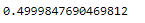
y_pred = lm.predict(x[:,np.newaxis])
df = pd.DataFrame({'Actual': y, 'Predicted': y_pred})
df.head()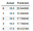
print('Mean Absolute Error:', metrics.mean_absolute_error(y, y_pred))
print('Mean Squared Error:', metrics.mean_squared_error(y, y_pred))
print('Root Mean Squared Error:', np.sqrt(metrics.mean_squared_error(y, y_pred)))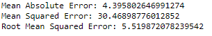
Conclusion: Poorer values than with the linear function. Let’s try exponential function.
6.2 Exponential Function
x = (cars["horsepower"]) ** 3
y = cars["mpg"]

lm = LinearRegression()
lm.fit(x[:,np.newaxis], y)
Calculation of R² and further parameters:
lm.score(x[:,np.newaxis], y)
y_pred = lm.predict(x[:,np.newaxis])
df = pd.DataFrame({'Actual': y, 'Predicted': y_pred})
df.head()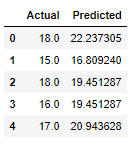
print('Mean Absolute Error:', metrics.mean_absolute_error(y, y_pred))
print('Mean Squared Error:', metrics.mean_squared_error(y, y_pred))
print('Root Mean Squared Error:', np.sqrt(metrics.mean_squared_error(y, y_pred)))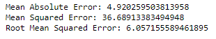
Conclusion: even worse values than in the previous two functions. Since the relationship looks non-linear, let’s try it with a log-transformation.
6.3 Logarithm Function
x = np.log(cars['horsepower'])
y = cars["mpg"]


lm = LinearRegression()
lm.fit(x[:,np.newaxis], y)
Calculation of R² and further parameters:
lm.score(x[:,np.newaxis], y)
y_pred = lm.predict(x[:,np.newaxis])
df = pd.DataFrame({'Actual': y, 'Predicted': y_pred})
df.head()
print('Mean Absolute Error:', metrics.mean_absolute_error(y, y_pred))
print('Mean Squared Error:', metrics.mean_squared_error(y, y_pred))
print('Root Mean Squared Error:', np.sqrt(metrics.mean_squared_error(y, y_pred)))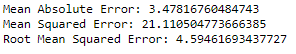
Conclusion: The model parameters have improved significantly with the use of the log function. Let’s see if we can further increase this with the polynomial function.
6.4 Polynomials Function
x = (cars["horsepower"])
y = cars["mpg"]

poly = PolynomialFeatures(degree=2)
x_ = poly.fit_transform(x[:,np.newaxis])

lm = linear_model.LinearRegression()
lm.fit(x_, y)
R²:
lm.score(x_, y)
Intercept and coefficients:
print(lm.intercept_)
print(lm.coef_)
The result can be interpreted as follows: mpg = 56,40 - 0,46 * horsepower + 0,001 * horsepower²
Further model parameters:
y_pred = lm.predict(x_)
df = pd.DataFrame({'Actual': y, 'Predicted': y_pred})
df.head()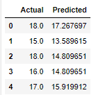
print('Mean Absolute Error:', metrics.mean_absolute_error(y, y_pred))
print('Mean Squared Error:', metrics.mean_squared_error(y, y_pred))
print('Root Mean Squared Error:', np.sqrt(metrics.mean_squared_error(y, y_pred)))
Now the degree of the polynomial function is increased until no improvement of the model can be recorded:
x = (cars["horsepower"])
y = cars["mpg"]

poly = PolynomialFeatures(degree=6)
x_ = poly.fit_transform(x[:,np.newaxis])
lm = linear_model.LinearRegression()
lm.fit(x_, y)
R²:
print(lm.score(x_, y))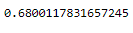
Intercept and coefficients:
print(lm.intercept_)
print(lm.coef_)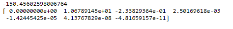
The result can be interpreted as follows: mpg = -150,46 + 1,07 * horsepower -2,34 * horsepower2 + 2,5 * horsepower3 - 1,42 * horsepower4 + 4,14 * horsepower5 - 4,82 * horsepower6
Further model parameters:
y_pred = lm.predict(x_)
df = pd.DataFrame({'Actual': y, 'Predicted': y_pred})
df.head()
print('Mean Absolute Error:', metrics.mean_absolute_error(y, y_pred))
print('Mean Squared Error:', metrics.mean_squared_error(y, y_pred))
print('Root Mean Squared Error:', np.sqrt(metrics.mean_squared_error(y, y_pred)))
7 Conclusion
In this post it was shown how model performance in non-linear contexts could be improved by using different transformation functions.
Finally, here is an overview of the created models and their parameters:
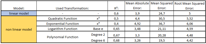
What these metrics mean and how to interpret them I have described in the following post: Metrics for Regression Analysis
Source
Kumar, A., & Babcock, J. (2017). Python: Advanced Predictive Analytics: Gain practical insights by exploiting data in your business to build advanced predictive modeling applications. Packt Publishing Ltd.