1 Introduction
Regression analyzes are very common and should therefore be mastered by every data scientist.
For this post the dataset House Sales in King County, USA from the statistic platform “Kaggle” was used. You can download it from my GitHub Repository.
2 Loading the libraries and the data
import pandas as pd
import numpy as np
import statsmodels.formula.api as smf
import matplotlib.pyplot as plt
from sklearn.linear_model import LinearRegression
from sklearn.model_selection import train_test_split
from sklearn import metrics
house_prices = pd.read_csv("path/to/file/house_prices.csv")3 Implementing linear regression with the statsmodel library
3.1 Simple linear Regression
Following, a simple linear regression with the variables ‘price’ and ‘sqft_living’ is to be performed.
HousePrices_SimplReg = house_prices[['price', 'sqft_living']]
HousePrices_SimplReg.head()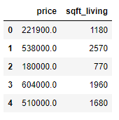
x = HousePrices_SimplReg['sqft_living']
y = HousePrices_SimplReg['price']

plt.scatter(x, y)
plt.title('Scatter plot: sqft_living vs. price')
plt.xlabel('sqft_living')
plt.ylabel('price')
plt.show()
model1 = smf.ols(formula='price~sqft_living', data=HousePrices_SimplReg).fit()The coefficients of the model are obtained in the following way:
model1.params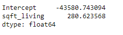
The result can be interpreted as follows: price = -43.580,74 + 280,62 * sqft_living
Hereby we get the R2:
model1.rsquared
With the summary function all model parameters can be displayed:
model1.summary()
With the perdict function, predictions can now be made based on the model created.
price_pred = model1.predict(pd.DataFrame(HousePrices_SimplReg['sqft_living']))For an assessment how well our model fits the data the following parameters are calculated:
HousePrices_SimplReg['price_pred'] = price_pred
HousePrices_SimplReg['RSE'] = (HousePrices_SimplReg['price'] - HousePrices_SimplReg['price_pred']) ** 2
RSEd = HousePrices_SimplReg.sum()['RSE']
RSE = np.sqrt(RSEd/21611)
criteria_mean = np.mean(HousePrices_SimplReg['price'])
error = RSE/criteria_mean
RSE, criteria_mean, error
Results of parameters:
- RSE = 261.452,89
- Mean of actal price = 540.088,14
- Ratio of RSE and criteria_mean = 48,41%
HousePrices_SimplReg.head()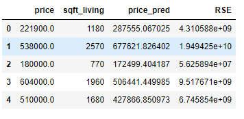
3.2 Multiple Regression
Now we try to improve the predictive power of the model by adding more predictors. Therefore we’ll have a look at the R-squared, the F-statistic and the Prob (F-statistic).
HousePrices_MultReg = house_prices[['price', 'sqft_living', 'bedrooms', 'yr_built']]
HousePrices_MultReg.head()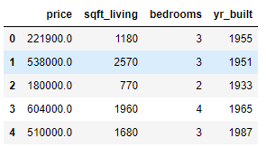
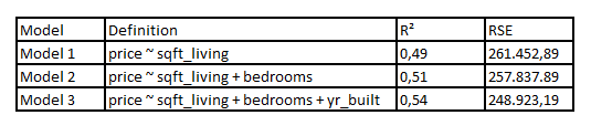
- Model 1: price ~ sqft_living
- Model 2: price ~ sqft_living + bedrooms
- Model 3: price ~ sqft_living + bedrooms + yr_built
model2 = smf.ols(formula='price~sqft_living+bedrooms', data=HousePrices_MultReg).fit()model2.params
model2.summary()
price_pred = model2.predict(HousePrices_MultReg[['sqft_living', 'bedrooms']])HousePrices_MultReg['price_pred'] = price_pred
HousePrices_MultReg['RSE'] = (HousePrices_MultReg['price'] - HousePrices_MultReg['price_pred']) ** 2
RSEd = HousePrices_MultReg.sum()['RSE']
RSE = np.sqrt(RSEd/21610)
criteria_mean = np.mean(HousePrices_MultReg['price'])
error = RSE/criteria_mean
RSE, criteria_mean, error
Results of parameters:
- RSE = 257.837.89
- Mean of actal price = 540.088.14
- Ratio of RSE and criteria_mean = 47,74%
HousePrices_MultReg.head()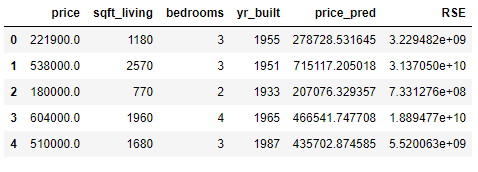
model3 = smf.ols(formula='price~sqft_living+bedrooms+yr_built', data=HousePrices_MultReg).fit()model3.params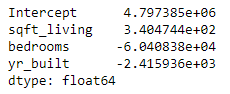
model3.summary()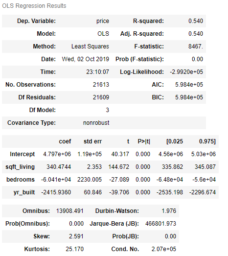
price_pred = model3.predict(HousePrices_MultReg[['sqft_living', 'bedrooms', 'yr_built']])HousePrices_MultReg['price_pred'] = price_pred
HousePrices_MultReg['RSE'] = (HousePrices_MultReg['price'] - HousePrices_MultReg['price_pred']) ** 2
RSEd = HousePrices_MultReg.sum()['RSE']
RSE = np.sqrt(RSEd/21609)
criteria_mean = np.mean(HousePrices_MultReg['price'])
error = RSE/criteria_mean
RSE, criteria_mean, error
Results of parameters:
- RSE = 248.923,19
- Mean of actal price = 540.088,14
- Ratio of RSE and criteria_mean = 46,09%
Below is an overview of the major results of the created models:
3.3 Model validation
We saw that model 3 delivered the best values. Therefore, our linear model is trained with this. Afterwards the performance will be measured.
a = np.random.randn(len(HousePrices_MultReg))
check = a < 0.8
training = HousePrices_MultReg[check]
testing = HousePrices_MultReg[~check]
print(training.shape)
print(testing.shape)
Let’s train our model
model4 = smf.ols(formula='price~sqft_living+bedrooms+yr_built', data=training).fit()
model4.summary()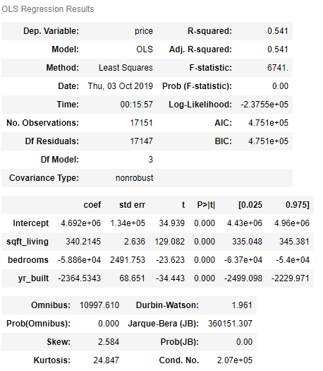
Now we use the trained model for the predictions:
price_pred = model4.predict(testing[['sqft_living', 'bedrooms', 'yr_built']])Check the model performance with the test data:
Important: For the calculation shown below, the Df residuals from the test record must be used. These can be determined as follows.
df_testing_model = smf.ols(formula='price~sqft_living+bedrooms+yr_built', data=testing).fit()
df_testing_model.summary()
Model performance:
testing['price_pred'] = price_pred
testing['RSE'] = (testing['price'] - testing['price_pred']) ** 2
RSEd = testing.sum()['RSE']
RSE = np.sqrt(RSEd/4458)
criteria_mean = np.mean(testing['price'])
error = RSE/criteria_mean
RSE, criteria_mean, error
Results of parameters:
- RSE = 242.210,56
- Mean of actal price = 534.152,74
- Ratio of RSE and criteria_mean = 45,34%
Both models are almost identical in comparison. However, the F-values are worse for the split model. This is normal because there was less data available for creating the model.
4 Linear Regression with scikit-learn
The library scikit-learn is also very good for training models. A brief insight should give the following example.
feature_cols = ['sqft_living', 'bedrooms', 'yr_built']
x = HousePrices_MultReg[feature_cols]
y = HousePrices_MultReg['price']
trainX, testX, trainY, testY = train_test_split(x, y, test_size = 0.2)
lm = LinearRegression()
lm.fit(trainX, trainY)
print(lm.intercept_)
print(lm.coef_)
The result can be interpreted as follows: price = 4.829.374,95 + 342,68 * sqft_living - 59.209,59 * bedrooms - 2.436,52 * yr_built
The coefficients can also be displayed more beautifully in the following two ways:
list(zip(feature_cols, lm.coef_))
coeff_df = pd.DataFrame(lm.coef_, feature_cols, columns=['Coefficient'])
coeff_df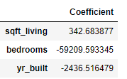
Calculation of R²:
lm.score(trainX, trainY)
y_pred = lm.predict(testX)df = pd.DataFrame({'Actual': testY, 'Predicted': y_pred})
df.head()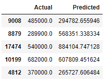
Now let’s plot the comparison of Actual and Predicted values
df1 = df.head(30)
df1.plot(kind='bar',figsize=(10,6))
plt.grid(which='major', linestyle='-', linewidth='0.5', color='green')
plt.grid(which='minor', linestyle=':', linewidth='0.5', color='black')
plt.show()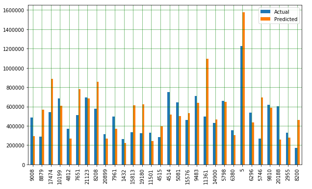
print('Mean Absolute Error:', metrics.mean_absolute_error(testY, y_pred))
print('Mean Squared Error:', metrics.mean_squared_error(testY, y_pred))
print('Root Mean Squared Error:', np.sqrt(metrics.mean_squared_error(testY, y_pred)))
What these metrics mean and how to interpret them I have described in the following post: Metrics for Regression Analysis
5 Conclusion
This was a small insight into the creation and use of linear regression models. In a subsequent post, the possible measures for the preparation of a linear model training will be shown. In a further contribution methods are to be shown how the predictive power of a linear model can be improved.
Source
Kumar, A., & Babcock, J. (2017). Python: Advanced Predictive Analytics: Gain practical insights by exploiting data in your business to build advanced predictive modeling applications. Packt Publishing Ltd.