1 Introduction

In the following posts, all possible machine learning algorithms will be shown promptly. In order to test their functionality in a superficial way, you do not necessarily have to look for a suitable data set (from the internet or similar). Because there is also the possibility to have an artificial data set created for the respective application needs. How this can be done I show in this post.

2 Import the libraries

from sklearn.datasets import make_regression
from sklearn.datasets import make_classification
from sklearn.datasets import make_blobs

from matplotlib import pyplot as plt

import pandas as pd
import numpy as np
import random

from drawdata import draw_scatter

3 Definition of required functions

def random_datetimes(start, end, n):
    '''
    Generates random datetimes in a certain range.
    
    Args:
        start (datetime): Datetime for which the range should start
        end (datetime): Datetime for which the range should end
        n (int): Number of random datetimes to be generated
    
    Returns:
        Randomly generated n datetimes within the defined range
    '''
    start_u = start.value//10**9
    end_u = end.value//10**9

    return pd.to_datetime(np.random.randint(start_u, end_u, n), unit='s')

4 Simulated Data

As already mentioned at the beginning, you can generate your own artificial data for each application. To do so we need the following libraries:

4.1 Make Simulated Data For Regression

features, output = make_regression(n_samples=100, n_features=1)

# plot regression dataset
plt.scatter(features,output)
plt.show()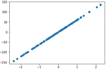

We can generate also more features:

features, output = make_regression(n_samples=100, n_features=4)

And safe these features to an object:

features = pd.DataFrame(features, columns=['Store_1', 'Store_2', 'Store_3', 'Store_4'])
features.head()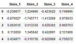

Now we do so for the output/target variable:

output = pd.DataFrame(output, columns=['Sales'])
output.head()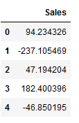

We also can combine these two objects to a final-dataframe:

df_final = pd.concat([features, output], axis=1)
df_final.head()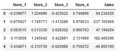

Now we are ready for using some machine learning or statistic models:

import statsmodels.api as sm

SM_model = sm.OLS(output, features).fit()
print(SM_model.summary())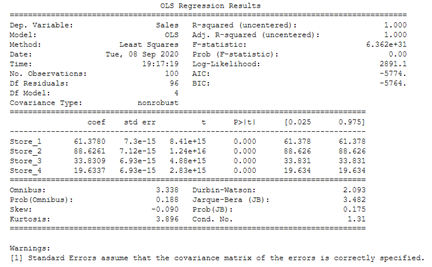

4.2 Make Simulated Data For Classification

With almost the same procedure we can also create data for classification tasks.

features, output = make_classification(n_samples=100, n_features=25)

pd.DataFrame(features).head()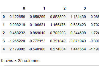

See here we have 25 features (=columns) and, by default, two output-classes:

pd.DataFrame(output, columns=['Target']).value_counts()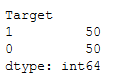

In the following I show two examples of how the characteristics of the artificially generated data can be changed:

features, output = make_classification(
                   n_samples=100, 
                   n_features=25,
                   flip_y=0.1)

# the default value for flip_y is 0.01, or 1%
# 10% of the values of Y will be randomly flipped

features, output = make_classification(
                   n_samples=100, 
                   n_features=25,
                   class_sep=0.1)

# the default value for class_sep is 1.0. The lower the value, the harder classification is

So far we have only created data sets that contain two classes (in the output variable). Of course, we can also create data sets for multi-classification tasks.

features, output = make_classification(n_samples=10000, n_features=10, n_informative=5, n_classes=5)

pd.DataFrame(output, columns=['Target']).value_counts()

4.3 Make Simulated Data For Clustering

Last but not least we’ll generate some data for cluster-problems.

X, y = make_blobs(n_samples=1000, n_features = 2, centers = 3, cluster_std = 0.7)

plt.scatter(X[:, 0], X[:, 1])
plt.xlabel("Feature 1")
plt.ylabel("Feature 2")
plt.show()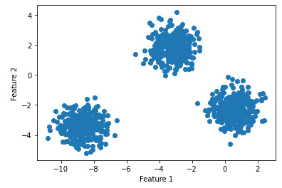

pd.DataFrame(X).head()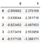

5 Customized dataset

df = pd.DataFrame({'Name': ['Maria', 'Marc', 'Julia'],
                   'Age': [32,22,62],
                   'Height': [162, 184, 170],
                   'Gender': ['female', 'male', 'female']})
df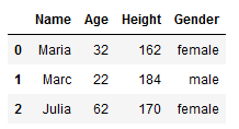

5.1 Insert a new row to pandas dataframe

5.1.1 In the first place

df.loc[-1] = ['Sven', 55, 181, 'male']  # adding a row
df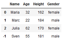

df.index = df.index + 1  # shifting index
df = df.sort_index()  # sorting by index
df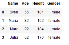

5.1.2 In the last place

The last index of our record is 3. Therefore, if we want to insert the new line at the end, we must now use .loc[4] in our case.

df.loc[4] = ['Max', 14, 175, 'male']  # adding a row
df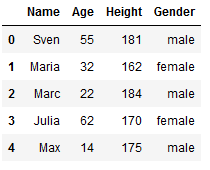

5.1.3 With a defined function

Here is a small function with the help of which you can easily add more rows to a record.

def insert(df, row):
    insert_loc = df.index.max()

    if pd.isna(insert_loc):
        df.loc[0] = row
    else:
        df.loc[insert_loc + 1] = row

insert(df,['Michael', 31, 182, 'male'])
df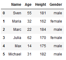

5.1.4 With the append function

df = df.append(pd.DataFrame([['Lisa', 34, 162, 'female']], columns=df.columns), ignore_index=True)
df.index = (df.index + 1) % len(df)
df = df.sort_index()
df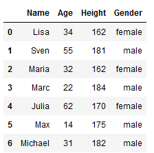

5.2 Insert a new column to pandas dataframe

Often you want to add more information to your artificially created dataset, such as randomly generated datetimes. This can be done as follows.

For this purpose, we continue to use the data set created in the previous chapter and extend it.

5.2.1 Random Dates

For this we use the function defined in chapter 3.

In the defined function we only have to enter the start and end date, as well as the length of the record (len(df)).

start = pd.to_datetime('2020-01-01')
end = pd.to_datetime('2020-12-31')

random_datetimes_list = random_datetimes(start, end, len(df))
random_datetimes_list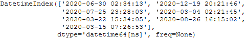

We can now add the list of generated datetimes to the dataset as a separate column.

df['date'] = random_datetimes_list
df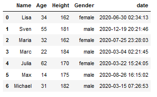

Here we go!

5.2.1 Random Integers

Of course, you also have the option to randomly generate integers. In the following I will show an example how to output integers in a certain range with defined steps:

Start = 40000
Stop = 120000
Step = 10000
Limit = len(df)

# List of random integers with Step parameter
rand_int_list = [random.randrange(Start, Stop, Step) for iter in range(Limit)]
rand_int_list

Just define Start, Stop and Step for your particular use. The Limit will be the length of the dataframe.

df['Salary'] = rand_int_list
df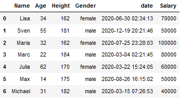

Now we also have a column for salary information in a range of 40k-120k with 10k steps.

5.3 Draw Data

Also a very useful thing is if you can draw the dataset yourself. Here the library ‘drawdata’ offers itself.

draw_scatter()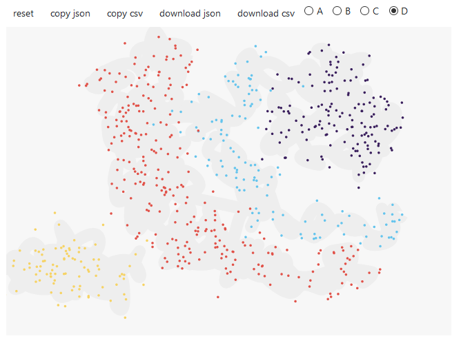

If you execute the command shown above, a blank sheet appears first. Now you have the possibility to draw 4 categories (A, B, C and D). More is unfortunately not yet possible, but is normally sufficient.

You only have to select one of the 4 categories and then you can draw your point clouds on the blank sheet.

Afterwards you have the possibility to save the drawn data as .csv or .json file:

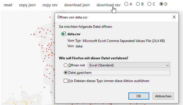
If you want to proceed without saving the data separately, click once on ‘copy csv’

and execute the following command:

new_df = pd.read_clipboard(sep=",")
new_df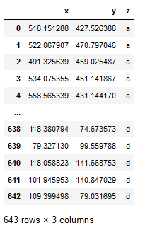

Now we can get started with the new data.

6 Conclusion

As you can see, the way in which artificial data is created basically always works the same. Of course, you can change the parameters accordingly depending on the application. See the individual descriptions on scikit-learn:

How to create artificial datasets