1 Introduction
Now that we have cleaned up and prepared our text dataset in the previous posts, we come to the next topic: Text Vectorization
Most machine learning algorithms cannot handle string variables. We have to convert them into a format that is readable for machine learning algorithms. Text vectorization is the process of converting text into real numbers. These numbers can be used as input to machine learning models.
In the following, I will use a simple example to show several ways in which vectorization can be done.
Finally, I will apply a vectorization method to the dataset (‘Amazon_Unlocked_Mobile_small_pre_processed.csv’) created and processed in the last post and train a machine learning model on it.
2 Import the Libraries and the Data
import pandas as pd
import numpy as np

from sklearn.feature_extraction.text import CountVectorizer
from sklearn.feature_extraction.text import TfidfVectorizer

from sklearn.model_selection import train_test_split
from sklearn.svm import SVC

from sklearn.metrics import confusion_matrix
from sklearn.metrics import accuracy_score
df = pd.DataFrame({'Rating': [2,5,3],
'Text': ["This is a brown horse",
"This horse likes to play",
"The horse is in the stable"]})
df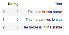
3 Text Vectorization
3.1 Bag-of-Words(BoW)
CountVectorizer() is one of the simplest methods of text vectorization.
It creates a sparse matrix consisting of a set of dummy variables. These indicate whether a certain word occurs in the document or not. The CountVectorizer function matches the word vocabulary, learns it, and creates a document term matrix where the individual cells indicate the frequency of that word in a given document. This is also called term frequency where the columns are dedicated to each word in the corpus.
3.1.2 Functionality
cv = CountVectorizer()

cv_vectorizer = cv.fit(df['Text'])
text_cv_vectorized = cv_vectorizer.transform(df['Text'])

text_cv_vectorized_array = text_cv_vectorized.toarray()

print(text_cv_vectorized_array)
print()
print(text_cv_vectorized_array.shape)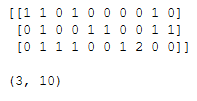
10 different words were found in the text corpus. These can also be output as follows:
cv_vectorizer.get_feature_names_out()
cv_vectorizer.vocabulary_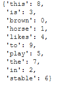
To make the output a bit more readable we can have it displayed as a dataframe:
cv_vectorized_matrix = pd.DataFrame(text_cv_vectorized.toarray(),
                                    columns=cv_vectorizer.get_feature_names_out())
cv_vectorized_matrix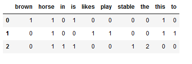
How are the rows and columns in the matrix shown above to be read?
- The rows indicate the documents in the corpus and
- The columns indicate the tokens in the dictionary
3.1.3 Creation of the final Data Set
Finally, I create a new data set on which to train machine learning algorithms. This time I use the generated array directly to create the final data frame:
cv_df = pd.DataFrame(text_cv_vectorized_array,
                     columns = cv_vectorizer.get_feature_names_out()).add_prefix('Counts_')

df_new_cv = pd.concat([df, cv_df], axis=1, sort=False)
df_new_cv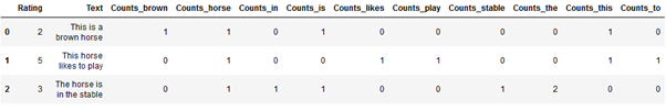
However, the bag-of-words method also has two crucial disadvantages:
- BoW does not preserve the order of words and
- It does not allow to draw useful conclusions for downstream NLP tasks
3.1.4 Test of a Sample Record
Let’s test a sample record:
new_input = ["Hi this is Mikel."]
new_input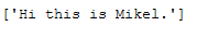
new_input_cv_vectorized = cv_vectorizer.transform(new_input)
new_input_cv_vectorized_array = new_input_cv_vectorized.toarray()
new_input_cv_vectorized_array
new_input_matrix = pd.DataFrame(new_input_cv_vectorized_array,
                                columns = cv_vectorizer.get_feature_names_out())

new_input_matrix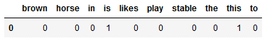
The words ‘is’ and ‘this’ have been learned by the CountVectorizer and thus get a count here.
new_input = ["You say goodbye and I say hello", "hello world"]
new_input
new_input_cv_vectorized = cv_vectorizer.transform(new_input)
new_input_cv_vectorized_array = new_input_cv_vectorized.toarray()
new_input_cv_vectorized_array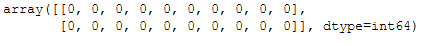
new_input_matrix = pd.DataFrame(new_input_cv_vectorized_array,
                                columns = cv_vectorizer.get_feature_names_out())

new_input_matrix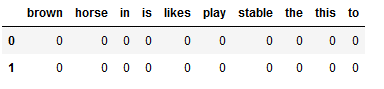
In our second example, I did not use any of the words CountVectorizer learned. Therefore all values are 0.
3.2 N-grams
3.2.1 Explanation
First of all, what are n-grams? In a nutshell: an N-gram means a sequence of N words. So for example, “Hi there” is a 2-gram (a bigram), “Hello sunny world” is a 3-gram (trigram) and “Hi this is Mikel” is a 4-gram.
How would this look when vectorizing a text corpus?
Example: “A horse rides on the beach.”
- Unigram (1-gram): A, horse, rides, on, the, beach
- Bigram (2-gram): A horse, horse rides, rides on, …
- Trigram (3-gram): A horse rides, horse rides on, …
Unlike BoW, n-gram maintains word order. They can also be created with the CountVectorizer() function. For this only the ngram_range parameter must be adjusted.
An ngram_range of:
- (1, 1) means only unigrams
- (1, 2) means unigrams and bigrams
- (2, 2) means only bigrams
- (1, 3) means unigrams, bigrams and trigrams …
Here a short example of this:
example_sentence = ["A horse rides on the beach."]
example_sentence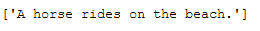
cv_ngram = CountVectorizer(ngram_range=(1, 3))

cv_ngram_vectorizer = cv_ngram.fit(example_sentence)
cv_ngram_vectorizer.get_feature_names_out()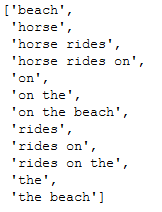
cv_ngram = CountVectorizer(ngram_range=(2, 3))

cv_ngram_vectorizer = cv_ngram.fit(example_sentence)
cv_ngram_vectorizer.get_feature_names_out()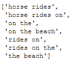
3.2.2 Functionality
3.2.2.1 Defining ngram_range
Now that we know how the CountVectorizer works with the ngram_range parameter, we will apply it to our sample dataset:
cv_ngram = CountVectorizer(ngram_range=(1, 3))

cv_ngram_vectorizer = cv_ngram.fit(df['Text'])
text_cv_ngram_vectorized = cv_ngram_vectorizer.transform(df['Text'])

text_cv_ngram_vectorized_array = text_cv_ngram_vectorized.toarray()

print(cv_ngram_vectorizer.get_feature_names_out())
The disadvantage of n-gram is that it usually generates too many features and is therefore very computationally expensive. One way to counteract this is to limit the maximum number of features. This can be done with the max_features parameter.
3.2.2.2 Defining max_features
cv_ngram = CountVectorizer(ngram_range=(1, 3),
                           max_features=15)

cv_ngram_vectorizer = cv_ngram.fit(df['Text'])
text_cv_ngram_vectorized = cv_ngram_vectorizer.transform(df['Text'])

text_cv_ngram_vectorized_array = text_cv_ngram_vectorized.toarray()

print(cv_ngram_vectorizer.get_feature_names_out())
cv_ngram_vectorized_matrix = pd.DataFrame(text_cv_ngram_vectorized.toarray(),
                                          columns=cv_ngram_vectorizer.get_feature_names_out())
cv_ngram_vectorized_matrix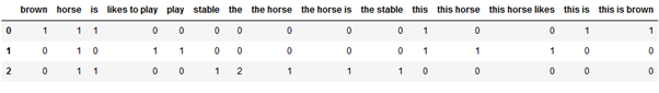
That worked out well. But what I always try to avoid with column names are spaces between the words. But this can be easily corrected:
cv_ngram_vectorized_matrix_columns_list = cv_ngram_vectorized_matrix.columns.to_list()

k = []

for i in cv_ngram_vectorized_matrix_columns_list:
    j = i.replace(' ','_')
    k.append(j)

cv_ngram_vectorized_matrix.columns = [k]
cv_ngram_vectorized_matrix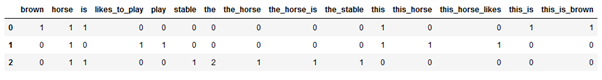
3.2.3 Creation of the final Data Set
cv_ngram_df = pd.DataFrame(text_cv_ngram_vectorized_array,
                           columns = cv_ngram_vectorizer.get_feature_names_out()).add_prefix('Counts_')

df_new_cv_ngram = pd.concat([df, cv_ngram_df], axis=1, sort=False)
df_new_cv_ngram.T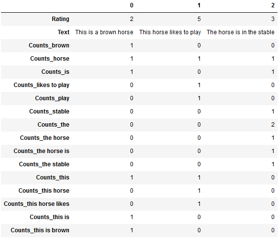
3.3 TF-IDF
3.3.1 Explanation
TF-IDF stands for Term Frequency - Inverse Document Frequency . It’s a statistical measure of how relevant a word is with respect to a document in a collection of documents.
TF-IDF consists of two components:
- Term frequency (TF): The number of times the word occurs in the document
- Inverse Document Frequency (IDF): A weighting that indicates how common or rare a word is in the overall document set.
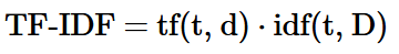
Multiplying TF and IDF results in the TF-IDF score of a word in a document. The higher the score, the more relevant that word is in that particular document.
3.3.1.1 Mathematical Formulas
TF-IDF is therefore the product of TF and IDF:
where TF computes the term frequency:
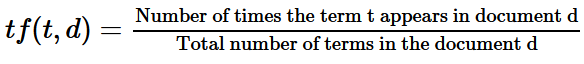
and IDF computes the inverse document frequency:

3.3.1.2 Example Calculation
Here is a simple example. Let’s assume we have the following collection of documents D:
- Doc1: “I said please and you said thanks”
- Doc2: “please darling please”
- Doc3: “please thanks”
The calculation of TF, IDF and TF-IDF is shown in the table below:
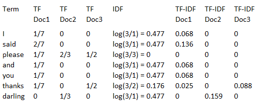
Let’s take a closer look at the values to understand the calculation. The word ‘said’ appears twice in the first document, and the total number of words in Doc1 is 7.
The TF value is therefore 2/7.
In the other two documents ‘said’ is not present at all. This results in an IDF value of log(3/1), since there are a total of three documents in the collection and the word ‘said’ appears in one of the three.
The calculation of the TF-IDF value is therefore as follows:
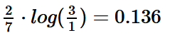
If you look at the values for ‘please’, you will see that this word appears (sometimes several times) in all documents. It is therefore considered common and receives a TF-IDF value of 0.
3.3.1.3 TF-IDF using scikit-learn
Below I will use the TF-IDF vectorizer from scikit-learn, which has two small modifications to the original formula.
The calculation of IDF is as follows:

Here, 1 is added to the numerator and to the denominator. This is to avoid the computational problem of dividing by 0. We also need to add a 1 to the numerator to balance the effect of adding 1 to the denominator.
The second modification is in the calculation of TF-IDF values:
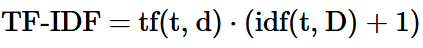
Here, a 1 is again added to IDF so that a zero value of IDF does not result in a complete suppression of TF-IDF. Using the TfidfVectorizer() function on our sample collection clearly shows this effect:
documents = ['I said please and you said thanks',
             'please darling please',
             'please thanks']

tf_idf = TfidfVectorizer()
tf_idf_vectorizer = tf_idf.fit(documents)
documents_tf_idf_vectorized = tf_idf_vectorizer.transform(documents)

documents_tf_idf_vectorized_array = documents_tf_idf_vectorized.toarray()


tf_idf_vectorized_matrix = pd.DataFrame(documents_tf_idf_vectorized.toarray(),
                                        columns=tf_idf_vectorizer.get_feature_names_out())
tf_idf_vectorized_matrix = tf_idf_vectorized_matrix[['said', 'please', 'and', 'you', 'thanks', 'darling']]
tf_idf_vectorized_matrix.T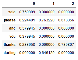
Here again for comparison the values calculated using the original formula:
As we can see here very nicely the values for the word ‘please’ were not completely suppressed during the calculation by TfidfVectorizer().
However, the interpretation of TF-IDF remain exactly the same despite these minor adjustments.
Furthermore, the word ‘I’ was not included, because scikit-learn’s vectorizer automatically disregards words with a length of one letter.
Hint:
Scikit-learn also provides the TfidfTransformer() function. But it needs the customized output of CountVectorize as input to calculate the TF-IDF values, see here. In almost all cases you can use TfidfVectorizer directly.
3.3.2 Functionality
tf_idf = TfidfVectorizer()
tf_idf_vectorizer = tf_idf.fit(df['Text'])
text_tf_idf_vectorized = tf_idf_vectorizer.transform(df['Text'])

text_tf_idf_vectorized_array = text_tf_idf_vectorized.toarray()


tf_idf_vectorized_matrix = pd.DataFrame(text_tf_idf_vectorized.toarray(),
                                        columns=tf_idf_vectorizer.get_feature_names_out())

tf_idf_vectorized_matrix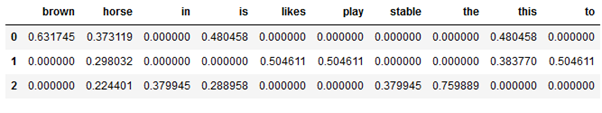
3.3.3 Creation of the final Data Set
tf_idf_df = pd.DataFrame(text_tf_idf_vectorized_array,
                         columns = tf_idf_vectorizer.get_feature_names_out()).add_prefix('TF-IDF_')

df_new_tf_idf = pd.concat([df, tf_idf_df], axis=1, sort=False)
df_new_tf_idf.T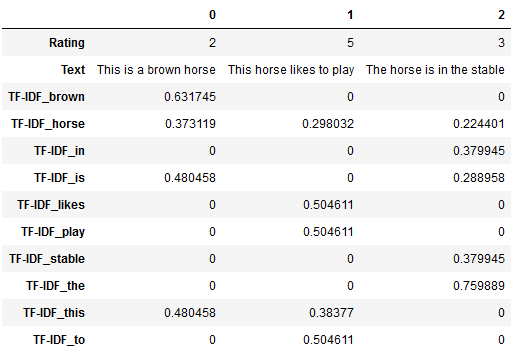
4 Best Practice - Application to the Amazon Data Set
As mentioned in the introduction, I will now apply a vectorizer to the dataset Amazon_Unlocked_Mobile_small_pre_processed.csv that I prepared in the last post. Afterwards, I will train a machine learning model on it.
Feel free to download the dataset from my GitHub Repository.
4.1 Import the Dataframe
url = "https://raw.githubusercontent.com/MFuchs1989/Datasets-and-Miscellaneous/main/datasets/NLP/Text%20Pre-Processing%20-%20All%20in%20One/Amazon_Unlocked_Mobile_small_pre_processed.csv"

df_amazon = pd.read_csv(url, error_bad_lines=False)
# Conversion of the desired column to the correct data type
df_amazon['Reviews_cleaned_wo_rare_words'] = df_amazon['Reviews_cleaned_wo_rare_words'].astype('str')
df_amazon.head(3).T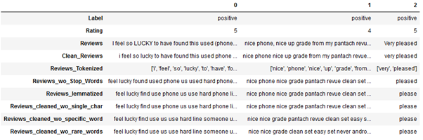
I have already prepared the data set in various ways. You can read about the exact steps here: NLP - Text Pre-Processing - All in One
I will apply the TF-IDF vectorizer to the ‘Reviews_cleaned_wo_rare_words’ column. For this I will create a subset of the original dataframe. Feel free to try the TF-IDF (or any other vectorizer) on the other processed columns and compare the performance of the ML algorithms.
df_amazon_subset = df_amazon[['Label', 'Reviews_cleaned_wo_rare_words']]
df_amazon_subset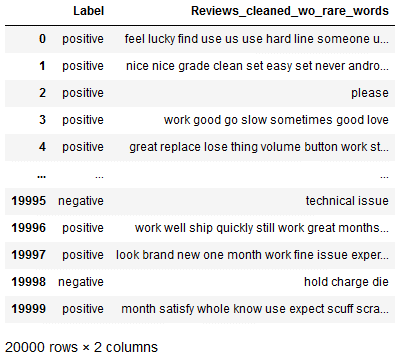
x = df_amazon_subset.drop(['Label'], axis=1)
y = df_amazon_subset['Label']

trainX, testX, trainY, testY = train_test_split(x, y, test_size = 0.2)
4.2 TF-IDF Vectorizer
As with scaling or encoding, the .fit command is applied only to the training part. Using these stored metrics, trainX as well as testX is then vectorized.
I still used the additional function .values.astype('U') in the code below. This would not have been necessary at this point, because I already assigned the correct data type to the column ‘Reviews_cleaned_wo_rare_words’ when loading the dataset.
To be on the safe side that TfidfVectorizer works, this code part can be kept.
tf_idf = TfidfVectorizer()
tf_idf_vectorizer = tf_idf.fit(trainX['Reviews_cleaned_wo_rare_words'].values.astype('U'))

trainX_tf_idf_vectorized = tf_idf_vectorizer.transform(trainX['Reviews_cleaned_wo_rare_words'].values.astype('U'))
testX_tf_idf_vectorized = tf_idf_vectorizer.transform(testX['Reviews_cleaned_wo_rare_words'].values.astype('U'))


trainX_tf_idf_vectorized_array = trainX_tf_idf_vectorized.toarray()
testX_tf_idf_vectorized_array = testX_tf_idf_vectorized.toarray()

print('Number of features generated: ' + str(len(tf_idf_vectorizer.get_feature_names_out())))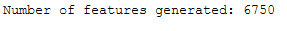
The next step is actually not necessary, since the machine learning models can handle arrays wonderfully.
trainX_tf_idf_vectorized_final = pd.DataFrame(trainX_tf_idf_vectorized_array,
                                              columns = tf_idf_vectorizer.get_feature_names_out()).add_prefix('TF-IDF_')

testX_tf_idf_vectorized_final = pd.DataFrame(testX_tf_idf_vectorized_array,
                                             columns = tf_idf_vectorizer.get_feature_names_out()).add_prefix('TF-IDF_')
4.3 Model Training
In the following I will use the Support Vector Machine classifier. Of course you can also try any other one.
clf = SVC(kernel='linear')
clf.fit(trainX_tf_idf_vectorized_final, trainY)

y_pred = clf.predict(testX_tf_idf_vectorized_final)
confusion_matrix = confusion_matrix(testY, y_pred)
print(confusion_matrix)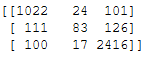
print('Accuracy: {:.2f}'.format(accuracy_score(testY, y_pred)))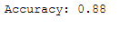
4.4 TF-IDF Vectorizer with ngram_range
The TF-IDF Vectorizer can also be used in combination with n-grams. It has been shown in practice that the use of the parameter analyser='char' in combination with ngram_range not only generates fewer features, which is less computationally intensive, but also often provides the better result.
tf_idf_ngram = TfidfVectorizer(analyzer='char',
                               ngram_range=(2, 3))

tf_idf_ngram_vectorizer = tf_idf_ngram.fit(trainX['Reviews_cleaned_wo_rare_words'].values.astype('U'))

trainX_tf_idf_ngram_vectorized = tf_idf_ngram_vectorizer.transform(trainX['Reviews_cleaned_wo_rare_words'].values.astype('U'))
testX_tf_idf_ngram_vectorized = tf_idf_ngram_vectorizer.transform(testX['Reviews_cleaned_wo_rare_words'].values.astype('U'))


trainX_tf_idf_ngram_vectorized_array = trainX_tf_idf_ngram_vectorized.toarray()
testX_tf_idf_ngram_vectorized_array = testX_tf_idf_ngram_vectorized.toarray()

print('Number of features generated: ' + str(len(tf_idf_ngram_vectorizer.get_feature_names_out())))
trainX_tf_idf_ngram_vectorized_final = pd.DataFrame(trainX_tf_idf_ngram_vectorized_array,
                                              columns = tf_idf_ngram_vectorizer.get_feature_names_out()).add_prefix('TF-IDF_ngram_')

testX_tf_idf_ngram_vectorized_final = pd.DataFrame(testX_tf_idf_ngram_vectorized_array,
                                              columns = tf_idf_ngram_vectorizer.get_feature_names_out()).add_prefix('TF-IDF_ngram_')
4.5 Model Training II
clf2 = SVC(kernel='linear')
clf2.fit(trainX_tf_idf_ngram_vectorized_final, trainY)

y_pred2 = clf2.predict(testX_tf_idf_ngram_vectorized_final)
y_pred2 = clf2.predict(testX_tf_idf_ngram_vectorized_final)confusion_matrix2 = confusion_matrix(testY, y_pred2)
print(confusion_matrix2)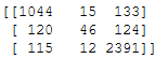
print('Accuracy: {:.2f}'.format(accuracy_score(testY, y_pred2)))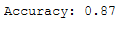
Unfortunately, the performance did not increase. Therefore, we use the first TF-IDF Vectorizer as well as the first ML model.
4.6 Out-Of-The-Box-Data
Finally, I’d like to test some self-generated evaluation comments and see what the model predicts.
Normally, all pre-processing steps that took place during model training should also be applied to new data. These were (to be read in the post NLP - Text Pre-Processing - All in One):
- Text Cleaning
- Conversion to Lower Case
- Removing HTML-Tags
- Removing URLs
- Removing Accented Characters
- Removing Punctuation
- Removing irrelevant Characters (Numbers and Punctuation)
- Removing extra Whitespaces
- Tokenization
- Removing Stop Words
- Normalization
- Removing Single Characters
- Removing specific Words
- Removing Rare words
For simplicity, I’ll omit these steps for this example, since I used simple words without punctuation or special characters.
my_rating_comment = ["a great device anytime again",
                     "has poor reception and a too small display",
                     "goes like this to some extent has a lot of good but also negative"]
Here is the vectorized data set:
my_rating_comment_vectorized = tf_idf_vectorizer.transform(my_rating_comment)
my_rating_comment_vectorized_array = my_rating_comment_vectorized.toarray()
my_rating_comment_df = pd.DataFrame(my_rating_comment_vectorized_array,
                                    columns = tf_idf_vectorizer.get_feature_names_out())
my_rating_comment_df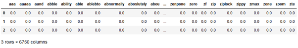
To be able to see which words from my_rating_comment were in the learned vocabulary of the vectorizer (and consequently received a TF-IDF score) I filter the dataset:
my_rating_comment_df_filtered = my_rating_comment_df.loc[:, (my_rating_comment_df != 0).any(axis=0)]
my_rating_comment_df_filtered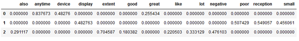
Ok let’s predict:
y_pred_my_rating = clf.predict(my_rating_comment_df)Here is the final result:
my_rating_comment_df_final = pd.DataFrame (my_rating_comment, columns = ['My_Rating'])
my_rating_comment_df_final['Prediction'] = y_pred_my_rating
my_rating_comment_df_final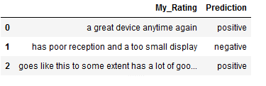
5 Conclusion
In this post I showed how to generate readable input from text data for machine learning algorithms. Furthermore, I applied a vectorizer to the previously created and cleaned dataset and trained a machine learning model on it. Finally, I showed how to make new predictions using the trained model.