1 Introduction
I have focused heavily on the topic of Text Pre-Processing in my past publications. At this point, I would like to summarize all the important steps in one post. Here I will not go into the theoretical background. For that, please read my earlier posts, where I explained in detail what I did and why.
For this publication the dataset Amazon Unlocked Mobile from the statistic platform “Kaggle” was used. You can download it from my “GitHub Repository”.
2 Import the Libraries and the Data
As you have seen in my past posts, I have written some useful functions for text pre-processing. Since my notebook would look pretty cluttered if I listed all the functions here, I created a separate .py file that contains all the featured functions. Feel free to download it from my “GitHub Repository”.
Below I will call some of these functions from the .py file and use them in this post.
import pandas as pd

import warnings
warnings.filterwarnings("ignore")

import matplotlib.pyplot as plt

from text_pre_processing import remove_html_tags_func
from text_pre_processing import remove_url_func
from text_pre_processing import remove_accented_chars_func
from text_pre_processing import remove_punctuation_func
from text_pre_processing import remove_irr_char_func
from text_pre_processing import remove_extra_whitespaces_func
from text_pre_processing import word_count_func
from text_pre_processing import word_tokenize
from text_pre_processing import remove_english_stopwords_func
from text_pre_processing import norm_lemm_v_a_func
from text_pre_processing import remove_single_char_func
from text_pre_processing import most_common_word_func
from text_pre_processing import least_common_word_func
from text_pre_processing import single_word_remove_func
from text_pre_processing import multiple_word_remove_func
from text_pre_processing import most_rare_word_func


pd.set_option('display.max_colwidth', 30)
df = pd.read_csv('Amazon_Unlocked_Mobile_small.csv')
df = df[['Rating', 'Reviews']]
df['Reviews'] = df['Reviews'].astype(str)
df.head()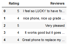
3 Text Pre-Processing
3.1 Text Cleaning
First, we perform some text cleaning steps. These are:
- Conversion to Lower Case
- Removing HTML-Tags
- Removing URLs
- Removing Accented Characters
- Removing Punctuation
- Removing irrelevant Characters (Numbers and Punctuation)
- Removing extra Whitespaces
df['Clean_Reviews'] = df['Reviews'].str.lower()
df['Clean_Reviews'] = df['Clean_Reviews'].apply(remove_html_tags_func)
df['Clean_Reviews'] = df['Clean_Reviews'].apply(remove_url_func)
df['Clean_Reviews'] = df['Clean_Reviews'].apply(remove_accented_chars_func)
df['Clean_Reviews'] = df['Clean_Reviews'].apply(remove_punctuation_func)
df['Clean_Reviews'] = df['Clean_Reviews'].apply(remove_irr_char_func)
df['Clean_Reviews'] = df['Clean_Reviews'].apply(remove_extra_whitespaces_func)

df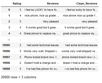
3.2 Tokenization
df['Reviews_Tokenized'] = df['Clean_Reviews'].apply(word_tokenize)

df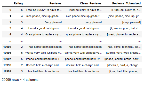
3.3 Stop Words
df['Reviews_wo_Stop_Words'] = df['Reviews_Tokenized'].apply(remove_english_stopwords_func)

df
3.4 Normalization
df['Reviews_lemmatized'] = df['Reviews_wo_Stop_Words'].apply(norm_lemm_v_a_func)

df.head(3).T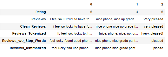
3.5 Removing Single Characters
df['Reviews_cleaned_wo_single_char'] = df['Reviews_lemmatized'].apply(remove_single_char_func)

df.head(3).T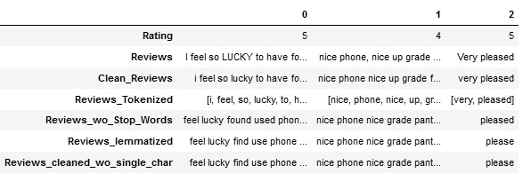
3.6 Text Exploration
3.6.1 Most common Words
3.6.1.1 for the whole DF
text_corpus = df['Reviews_cleaned_wo_single_char'].str.cat(sep=' ')

df_most_common_words_text_corpus = most_common_word_func(text_corpus)

df_most_common_words_text_corpus.head(10)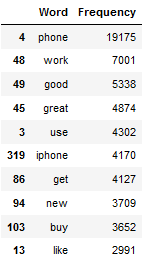
plt.figure(figsize=(11,7))
plt.bar(df_most_common_words_text_corpus['Word'],
        df_most_common_words_text_corpus['Frequency'])

plt.xticks(rotation = 45)

plt.xlabel('Most common Words')
plt.ylabel("Frequency")
plt.title("Frequency distribution of the 25 most common words")

plt.show()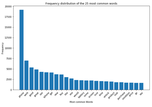
3.6.1.2 for parts of the DF
def label_func(rating):
    if rating <= 2:
        return 'negative'
    if rating >= 4:
        return 'positive'
    else:
        return 'neutral'

df['Label'] = df['Rating'].apply(label_func)
cols = list(df.columns)
cols = [cols[-1]] + cols[:-1]
df = df[cols]positive_review = df[(df["Label"] == 'positive')]['Reviews_cleaned_wo_single_char']
neutral_review = df[(df["Label"] == 'neutral')]['Reviews_cleaned_wo_single_char']
negative_review = df[(df["Label"] == 'negative')]['Reviews_cleaned_wo_single_char']text_corpus_positive_review = positive_review.str.cat(sep=' ')
text_corpus_neutral_review = neutral_review.str.cat(sep=' ')
text_corpus_negative_review = negative_review.str.cat(sep=' ')df_most_common_words_text_corpus_positive_review = most_common_word_func(text_corpus_positive_review)
df_most_common_words_text_corpus_neutral_review = most_common_word_func(text_corpus_neutral_review)
df_most_common_words_text_corpus_negative_review = most_common_word_func(text_corpus_negative_review)splited_data = [df_most_common_words_text_corpus_positive_review,
df_most_common_words_text_corpus_neutral_review,
df_most_common_words_text_corpus_negative_review]
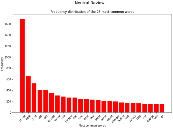
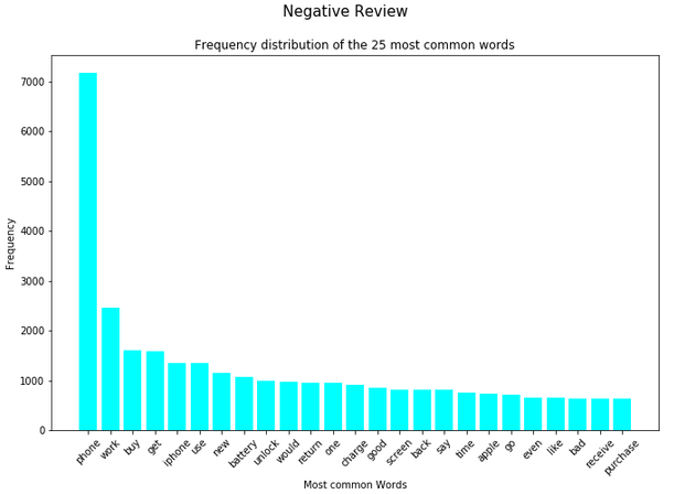
color_list = ['green', 'red', 'cyan']
title_list = ['Positive Review', 'Neutral Review', 'Negative Review']
for item in range(3):
plt.figure(figsize=(11,7))
plt.bar(splited_data[item]['Word'],
splited_data[item]['Frequency'],
color=color_list[item])
plt.xticks(rotation = 45)
plt.xlabel('Most common Words')
plt.ylabel("Frequency")
plt.title("Frequency distribution of the 25 most common words")
plt.suptitle(title_list[item], fontsize=15)
plt.show()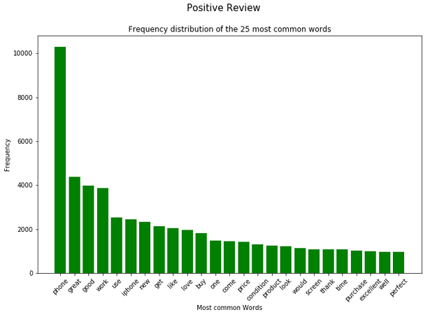
3.6.2 Least common Words
df_least_common_words_text_corpus = least_common_word_func(text_corpus, n_words=2500)

df_least_common_words_text_corpus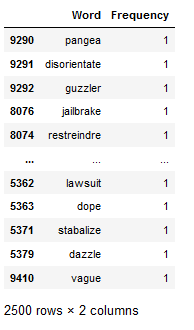
Let’s see if the 2,500 different words actually occur only once in the entire text corpus.
df_least_common_words_text_corpus[(df_least_common_words_text_corpus["Frequency"] > 1)].shape[0] 
3.7 Removing specific Words
In the analysis from the previous chapter, we saw that the word ‘phone’ occurs very frequently both in the total and in the dataset split by rating. For this reason, this word is excluded in a newly generated column.
df["Reviews_cleaned_wo_specific_word"] = df.apply(lambda x: single_word_remove_func(x["Reviews_cleaned_wo_single_char"],
                                                            "phone"), axis = 1)

df.head(3).T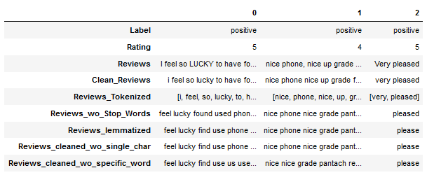
3.8 Removing Rare words
Furthermore, the analysis from the previous chapter revealed that at least 2,500 words occur only once in the entire text corpus of the ‘Reviews_cleaned_wo_single_char’ column. In order to be able to check later whether these words are profitable or not, I generate a new column without these 2,500 words.
most_rare_words_list_DataFrame = most_rare_word_func(text_corpus, n_words=2500)

df["Reviews_cleaned_wo_rare_words"] = df.apply(lambda x: multiple_word_remove_func(x["Reviews_cleaned_wo_specific_word"],
                                                         most_rare_words_list_DataFrame), axis = 1)
3.9 Final Results
The final data set looks like this:
df.head(3).T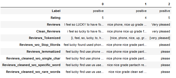
Here we generated three columns that presumably have different information densities.
On the one hand we have the column ‘Reviews_cleaned_wo_single_char’ where we have only applied all necessary pre-processing steps.
Then we have another column (‘Reviews_cleaned_wo_specific_word’) where we excluded the word ‘phone’.
Finally, we generated the column ‘Reviews_cleaned_wo_rare_words’, where we excluded the word ‘phone’ and 2,500 other words that occurred only once in the entire text corpus.
Now we need to vectorize the individual text columns to make them usable for machine learning algorithms. The validation of the model performance of the individual algorithms will then reveal which text column is most profitable for the analysis. It may be necessary to further adjust the columns if, for example, it turns out that the removal of rare words was very profitable.
I will describe this in detail in further posts.
4 Conclusion
In this post I have presented all possible text pre-processing steps, most of which I had also described in more detail in my post series on text pre-processing.
In order to be able to continue working with the edited data set at a later point in time, I now save it:
df.to_csv('Amazon_Unlocked_Mobile_small_pre_processed.csv', index = False)You can also download this edited dataset from my “GitHub Repository”