1 Introduction

After having developed a simple “Knowledge-based Recommender” we now come to another recommender: the Plot Description-based Recommender.

For this post the dataset movies_metadata from the statistic platform “Kaggle” was used. You can download it from my “GitHub Repository”.

2 Import the libraries and the data

import pandas as pd
import numpy as np

import preprocessing_recommender_systems as prs

from sklearn.feature_extraction.text import TfidfVectorizer
from sklearn.metrics.pairwise import linear_kernel

We are going to use the same dataframe as in the previous post.

df = pd.read_csv('movies_metadata.csv')
df.head()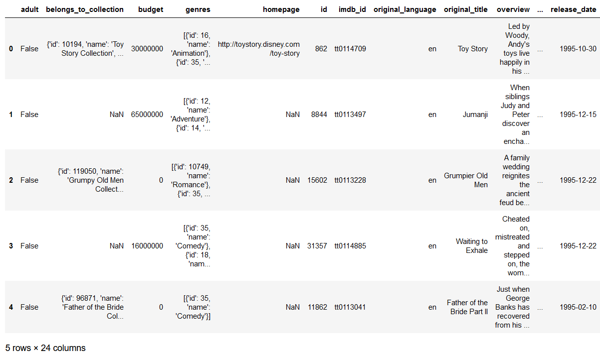

Some pre-processing steps are similar to those of the “Knowledge-based Recommender”. Since I don’t want to list them one by one again I have written them into a separate python file (preprocessing_recommender_systems.py). This file is also stored on my “GitHub Account” and can be downloaded from there.

3 Data pre-processing Part I

The process steps can be traced individually in Post “Knowledge-based Recommender” up to and including Chapter 3.2. The only difference is that we additionally keep the columns ‘overview’ and ‘id’.

df = prs.clean_data(df)
df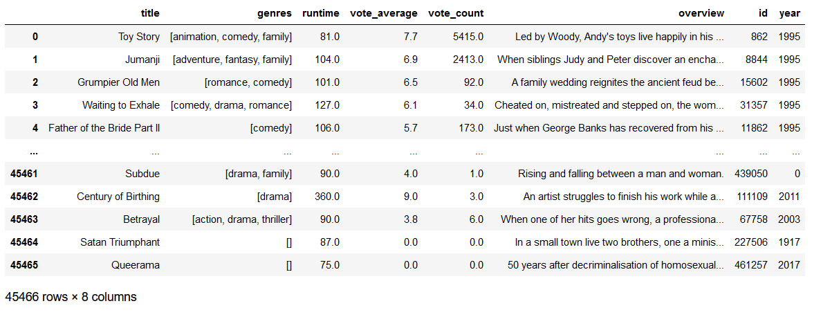

4 Data pre-processing Part II

The recommendation model I want to develop will be based on the pairwise similarity between bodies of text. But how do we numerically quantify the similarity between two bodies of text? The answer is Vectorizing.

4.1 Introduction of the CountVectorizer

The CountVectorizer is the simplest vectorizer and is best explained with the help of an example:

d = {'Line': [1, 2, 3], 'Text': ['The sun is a star', 'My love is like a red, red rose', 'Mary had a little lamb']}
test = pd.DataFrame(data=d)
test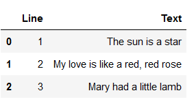

In the following we will convert the column text on the test dataset into its vector form. The first step is to calculate the size of the vocabulary. The vocabulary is the is the number of unique words present across all text rows. Due to the fact that the sentences contain some words that are not meaningful (so-called stop words) they are removed from the vocabulary.

#Import CountVectorizer from the scikit-learn library
from sklearn.feature_extraction.text import CountVectorizer

#Define a CountVectorizer Object. Remove all english stopwords
vectorizer = CountVectorizer(stop_words='english')

#Construct the CountVectorizer matrix
vectorizer_matrix = vectorizer.fit_transform(test['Text'])
vectorizer_matrix.shape

feature_names = vectorizer.get_feature_names()
print(feature_names)
print()
print('Length of vocabulary: ' + str(len(feature_names)))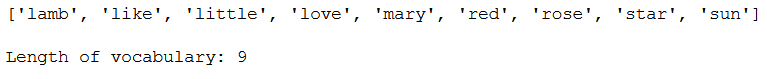

As we can see the length of the vocabulary is now 9.

result_vectorizer = pd.DataFrame(vectorizer_matrix.toarray(), columns = vectorizer.get_feature_names())
result_vectorizer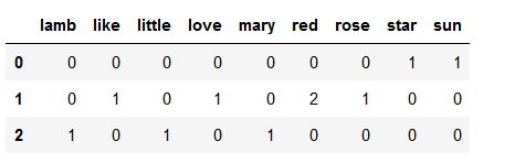

The overview can now be interpreted as follows:

The first dimension will represent the number if times the word ‘lamb’ occurs, the second will represent the number of times the word ‘like’ occurs and so on.

4.2 Introduction of the TF-IDFVectorizer

Not all words in a document carry equal weight. If you want to consider the weighting you should use the TF-IDFVectorizer. The syntax of the TF-IDFVectorizer is almost identical:

#Import TfIdfVectorizer from the scikit-learn library
from sklearn.feature_extraction.text import TfidfVectorizer

#Define a TF-IDF Vectorizer Object. Remove all english stopwords
tfidf = TfidfVectorizer(stop_words='english')

#Construct the TF-IDF matrix
tfidf_matrix = tfidf.fit_transform(test['Text'])
tfidf_matrix.shape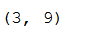

feature_names = tfidf.get_feature_names()
feature_names

result_tfidf = pd.DataFrame(tfidf_matrix.toarray(), columns = tfidf.get_feature_names())
result_tfidf

4.3 Create TF-IDF vectors

Let us return to our original data set after this short digression and apply here the TF-IDF to our movie dataset.

#Import TfIdfVectorizer from the scikit-learn library
from sklearn.feature_extraction.text import TfidfVectorizer

#Define a TF-IDF Vectorizer Object. Remove all english stopwords
tfidf = TfidfVectorizer(stop_words='english')

#Replace NaN with an empty string
df['overview'] = df['overview'].fillna('')

#Construct the required TF-IDF matrix by applying the fit_transform method on the overview feature
tfidf_matrix = tfidf.fit_transform(df['overview'])

#Output the shape of tfidf_matrix
tfidf_matrix.shape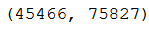

4.4 Compute the pairwise cosin similarity

# Import linear_kernel to compute the dot product
from sklearn.metrics.pairwise import linear_kernel

# Compute the cosine similarity matrix
cosine_sim = linear_kernel(tfidf_matrix, tfidf_matrix)

The cosin score can take any value between -1 and 1. The higher the cosin score, the more similar the documents are to each other. Now it’s time to build the Plot Description-based Recommender.

5 Build the Plot Description-based Recommender

#Construct a reverse mapping of indices and movie titles, and drop duplicate titles, if any
indices = pd.Series(df.index, index=df['title']).drop_duplicates()
indices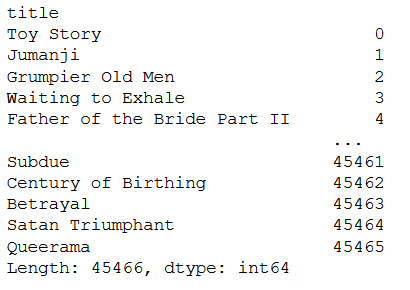

# Function that takes in movie title as input and gives recommendations 
def content_recommender(title, cosine_sim=cosine_sim, df=df, indices=indices):
    # Obtain the index of the movie that matches the title
    idx = indices[title]

    # Get the pairwsie similarity scores of all movies with that movie
    # And convert it into a list of tuples as described above
    sim_scores = list(enumerate(cosine_sim[idx]))

    # Sort the movies based on the cosine similarity scores
    sim_scores = sorted(sim_scores, key=lambda x: x[1], reverse=True)

    # Get the scores of the 10 most similar movies. Ignore the first movie.
    sim_scores = sim_scores[1:11]

    # Get the movie indices
    movie_indices = [i[0] for i in sim_scores]

    # Return the top 10 most similar movies
    return df['title'].iloc[movie_indices]

6 Test the recommender

Now we are going to test the recommender. Let’s have a look for similar movies for Toy Story.

#Get recommendations for Toy Story
content_recommender('Toy Story')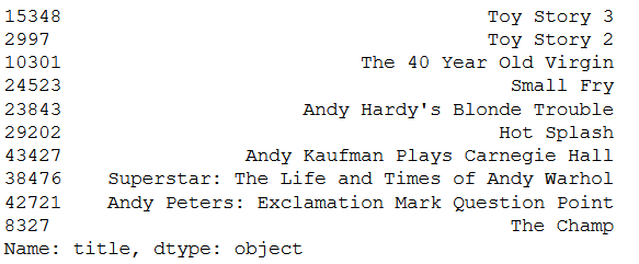

7 Conclusion

In this post I talked about creating a Plot Description-based Recommender. Compared to the Knowledge-based Recommender this has the advantage that it suggests movies that the user may not know from their content but have a strong relation to each other according to our similarity matrix.

References

The content of the entire post was created using the following sources:

Banik, R. (2018). Hands-On Recommendation Systems with Python: Start building powerful and personalized, recommendation engines with Python. Birmingham: Packt Publishing Ltd.

Recommendation Systems - Plot Description-based Recommender