1 Introduction
In marketing, customer lifetime value is one of the most important metrics to keep in mind. This metric is especially important to keep track of for acquiring new customers. The corporate goal of marketing campaigns is always the acquisition of new customers under the premise of a positive ROI. For example, if the average CLV of our customer is 100€ and it only costs 50€ to acquire a new customer, then our business will be generating more revenue as we acquire new customers. If this is the other way around, our company is making losses. This is to be avoided and for this reason the CLV should always be observed.
There are multiple ways to calculate CLV. One way is to find the customer’s average purchase amount, purchase frequency and lifetime span to do a simple calculation to get the CLV.
Let us assume the following conditions:
- Customer’s average purchase amount: 100€
- Purchase frequency: 5 times per month
This makes an average value per month of 500€. Now let’s come to the lifetime span. One way to estimate a customer’s lifetime span is to look at the average monthly churn rate, which is the percentage of customers leaving and terminating the relationship with our business. We can estimate a customer’s lifetime span by dividing one by the churn rate. Assuming 5% of the churn rate, the estimated customer’s lifetime span is 20 years.
- Lifetime span: 20 years
This results in a total amount of 120,000€ (500€ x 20 years x 12 months).
Because we do not typically know the lifetime span of customers, we often try to estimate CLV over the course of a certain period (3 months, 12 months, 24 months …). And that is exactly what we will do in the following.
For this post the dataset Online Retail from the statistic platform “Kaggle” was used. You can download it from my “GitHub Repository”.
2 Import the libraries and the data
import pandas as pd
import numpy as np


import matplotlib.pyplot as plt
from sklearn.model_selection import train_test_split
from sklearn.linear_model import LinearRegression
from sklearn import metrics
df = pd.read_excel('Online Retail.xlsx', sheet_name='Online Retail')
df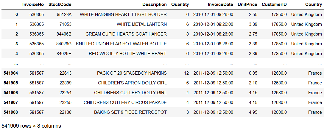
3 Data pre-processing
3.1 Negative Quantity
'''
Canceled orders could cause negative values in the data record.
To be on the safe side, these are removed.
'''

df = df.loc[df['Quantity'] > 0]
df.shape
As we can see from the output, this was not the case in this record.
3.2 Missing Values within CustomerID
'''
We need to drop observations with no CustomerID
'''

df = df[pd.notnull(df['CustomerID'])]
df.shape
3.3 Handling incomplete data
print('Invoice Date Range: %s - %s' % (df['InvoiceDate'].min(), df['InvoiceDate'].max()))
'''
Due to the fact that we only need full months for future analysis, we will shorten this data set accordingly.
'''

df = df.loc[df['InvoiceDate'] < '2011-12-01']
df.shape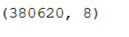
3.4 Total Sales
'''
For further analysis we need another column Sales.
'''
df['Sales'] = df['Quantity'] * df['UnitPrice']
df.head()
3.5 Create final dataframe
'''
Here we group the dataframe by CustimerID and InvoiceNo and
aggregate the Sales column as well as the InvoiceDate.
'''

orders_df = df.groupby(['CustomerID', 'InvoiceNo']).agg({
    'Sales': sum,
    'InvoiceDate': max
})

orders_df.head()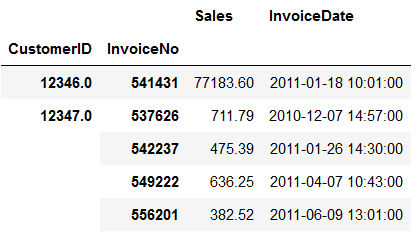
4 Descriptive Analytics
4.1 Final Dataframe for Descriptive Analytics
'''
For the preparation of the data for descriptive part we need the following functions:
'''


def groupby_mean(x):
    return x.mean()

def groupby_count(x):
    return x.count()

def purchase_duration(x):
    return (x.max() - x.min()).days

def avg_frequency(x):
    return (x.max() - x.min()).days/x.count()

groupby_mean.__name__ = 'avg'
groupby_count.__name__ = 'count'
purchase_duration.__name__ = 'purchase_duration'
avg_frequency.__name__ = 'purchase_frequency'
We re-group the record by CustomerID and aggregate the Sales and InvoiceDate columns with the previously created functions.
summary_df = orders_df.reset_index().groupby('CustomerID').agg({
    'Sales': [min, max, sum, groupby_mean, groupby_count],
    'InvoiceDate': [min, max, purchase_duration, avg_frequency]
})

summary_df.head()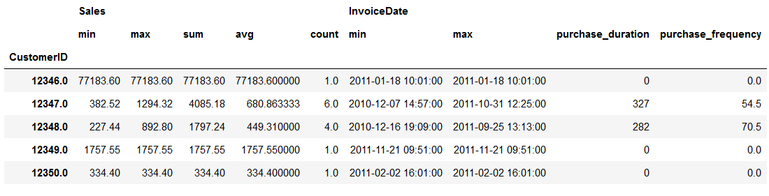
This still looks a bit messy now but we can / must make it a bit nicer.
summary_df.columns = ['_'.join(col).lower() for col in summary_df.columns]
summary_df = summary_df.reset_index()
summary_df.head()
This dataset gives us an idea of the purchases each customer has made. Let’s have a look at CustomerID 12346 (first row). This customer made only one purchase on January 18,2011.
The second customer (12347) has made six purchases within December 7, 2010 and October 31, 2011. The timespan here is about 327 days. The average amount this customer spent on each order is 680. We also see from the record, that this customer made a purchase every 54.5 days.
4.2 Visualizations
For the visualization part we are only interested in the purchases that the repeat customers have made.
summary_df = summary_df.loc[summary_df['invoicedate_purchase_duration'] > 0]
summary_df.shape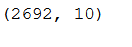
As we can see, there are only 2692 (of 4298) repeat customers in the record.
'''
This plot shows the distributions of the number of purchases that the repeat customers have made
'''

ax = summary_df.groupby('sales_count').count()['sales_avg'][:20].plot(
    kind='bar',
    color='skyblue',
    figsize=(12,7),
    grid=True
)

ax.set_ylabel('count')
plt.title('Number of purchases that the repeat customers have made')

plt.show()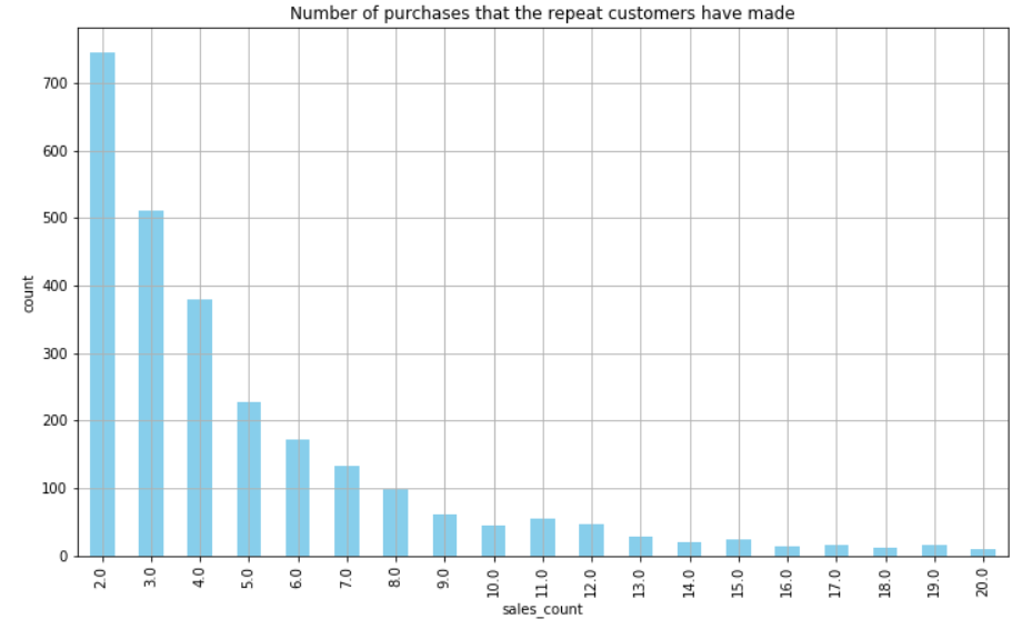
As we can see from this plot, the majority of customers have made 10 or less purchases. Here a few more metrics about sales_count:
summary_df['sales_count'].describe()
Now we are going to have a look at the average number of days between purchases for these repeat customers.
'''
This plot shows the average number of days between purchases for repeat customers.
It is an overall view of how frequently repeat customers made purchases historically.
'''

ax = summary_df['invoicedate_purchase_frequency'].hist(
    bins=20,
    color='skyblue',
    rwidth=0.7,
    figsize=(12,7)
)

ax.set_xlabel('avg. number of days between purchases')
ax.set_ylabel('count')
plt.title('Number of days between purchases for repeat customers')

plt.show()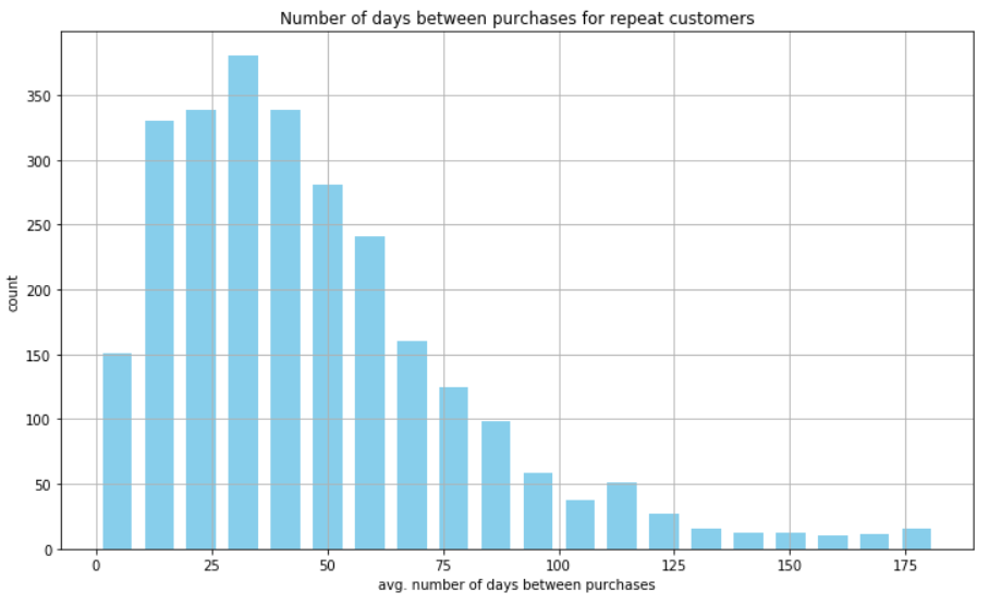
As we can see from this plot, the majority of repeat customers made purchases every 20-50 days.
5 Predicting 3-Month CLV
5.1 Final Dataframe for Prediction Models
We use the final created dataset orders_df at this point (chapter Data pre-processing / Create final dataframe)
# Determine the frequency
clv_freq = '3M'

# Group by CustomerID
# Break down the data into chunks of 3 months for each customer
# Aggregate the sales column by sum
# Aggregate the sales column by average_sum and count (both with the previous created functions)
data_df = orders_df.reset_index().groupby([
    'CustomerID',
    pd.Grouper(key='InvoiceDate', freq=clv_freq)
]).agg({
    'Sales': [sum, groupby_mean, groupby_count],
})

# Bring the dataset in a readable format
data_df.columns = ['_'.join(col).lower() for col in data_df.columns]
data_df = data_df.reset_index()
data_df.head()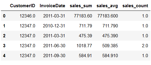
Now we are going to encode the InvoiceDate column values so that they are easier to read than the current date format.
# Set the length of the column InvoiceDate. In our case = 10
length_of_InvoiceDate = 10

date_month_map = {
    str(x)[:length_of_InvoiceDate]: 'M_%s' % (i+1) for i, x in enumerate(
        sorted(data_df.reset_index()['InvoiceDate'].unique(), reverse=True)
    )
}
date_month_map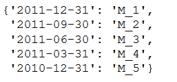
As you can see, we encoded the date values into M_1, M_2 and so on.
'''
Apply the generated dictionary to the dataframe for prediction models
'''

data_df['M'] = data_df['InvoiceDate'].apply(lambda x: date_month_map[str(x)[:length_of_InvoiceDate]])
data_df.head(10)
5.2 Building Sample Set
Now we are ready to create a sample set with features and target variables. In this case, we are going to use the last 3 months as the target variable and the rest as the features. In other words, we are going to train a machie learning model that predicts the last 3 months’customer value with the rest of the data.
# Exclude M_1 because this will be our predictor variable.
features_df = pd.pivot_table(
    data_df.loc[data_df['M'] != 'M_1'],
    values=['sales_sum', 'sales_avg', 'sales_count'],
    columns='M',
    index='CustomerID'
)

# Prepare the features dataframe for better view
features_df.columns = ['_'.join(col) for col in features_df.columns]

# Encode NaN values with 0.0
features_df = features_df.fillna(0)
features_df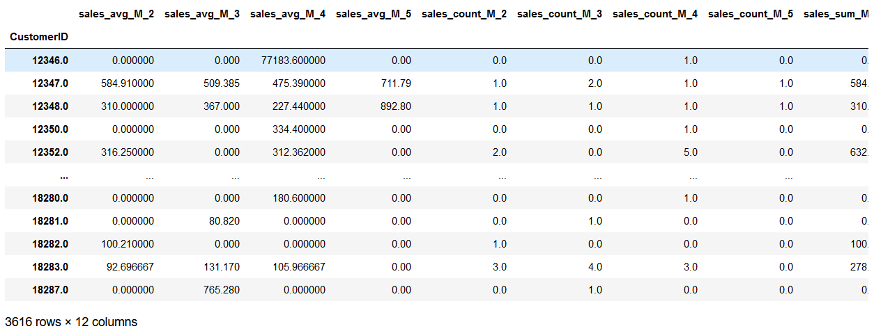
# Just select M_1 because this is our target variable
response_df = data_df.loc[
    data_df['M'] == 'M_1',
    ['CustomerID', 'sales_sum']
]

# Rename the columns accordingly
response_df.columns = ['CustomerID', 'CLV_'+clv_freq]
response_df
# Join the features_df and response_df  on CustomerID
sample_set_df = features_df.merge(
    response_df,
    left_index=True,
    right_on='CustomerID',
    how='left'
)

# Encode NaN values with 0.0
sample_set_df = sample_set_df.fillna(0)

sample_set_df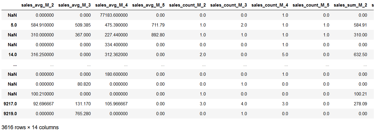
5.3 Train Test Split
target_var = 'CLV_'+clv_freq
all_features = [x for x in sample_set_df.columns if x not in ['CustomerID', target_var]]

print()
print('Target Variable: ' + str(target_var))
print()
print('----------------------------------------------------')
print()
print('Predictor Variables:')
print(all_features)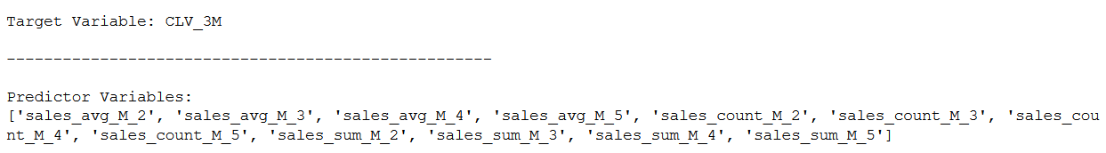
'''
Here we are going to do a train test split with a division of 70% to 30%.
'''

trainX, testX, trainY, testY  = train_test_split(
    sample_set_df[all_features],
    sample_set_df[target_var],
    test_size=0.3
)
5.4 Linear Regression
lm = LinearRegression()
lm.fit(trainX, trainY)
coef = pd.DataFrame(list(zip(all_features, lm.coef_)))
coef.columns = ['feature', 'Coefficient']
coef
Whith this overview we easily can see which features have negative or positive correlation with the target variable.
For example, the previous 3 month period’s average purchase amount, sales_avg_M_2 (line 1), has positive impacts on the next 3 month customer value. This means that the higher the previous 3 month period’s average purchase amount is, the higher the next 3 month purchase amount will be.
On the other hand, the second and third most recent 3 month period’s average purchase amounts, sales_avg_M_3 and sales_avg_M_4, are negatively correlated with the next 3 month customer value. In other words, the more a customer made purchases 3 months to 9 months ago, the lower value he or she will bring in the next 3 months.
5.5 Model Evaluation
y_pred = lm.predict(testX)

print('Mean Absolute Error:', metrics.mean_absolute_error(testY, y_pred))
print('Mean Squared Error:', metrics.mean_squared_error(testY, y_pred))
print('Root Mean Squared Error:', np.sqrt(metrics.mean_squared_error(testY, y_pred)))
6 Conclusion
In this post I have explained what the customer lifetime value is and how to run descriptive statistics on its underlying metrics.
I also showed how to prepare the data set for a three month prediction of the CLV and train a machine learning model.
I explained how to draw valuable conclusions about past periods from the results of the linear model and evaluate these insights.
Finally, I will say a few words about the advantages of such an analysis for a company:
Since you know the expected revenue or purchase amount from individual customers for the next 3 months, you can set a better informed budget for your marketing campaign. This should not be set too high but also not too low, so that the target customers are still reached but the ROI does not suffer.
On the other hand you can also use these 3 month customer value prediction output values to specifically target these high-value customers for the next 3 months. This can help you to create marketing campaigns with a higher ROI, as those high-value customers, predicted by the machine learning model, are likely to bring in more revenue than the others.
References
The content of the entire post was created using the following sources:
Hwang, Y. (2019). Hands-On Data Science for Marketing: Improve your marketing strategies with machine learning using Python and R. Packt Publishing Ltd.