1 Introduction
Another exciting topic in marketing analytics is Market Basket Analysis. This is the topic of this publication. At the beginning of this post I will be introducing some key terms and metrics aimed at giving a sense of what “association” in a rule means and some ways to quantify the strength of this association. Then I will show how to generate these rules from the dataset ‘Online Retail’ using the Apriori Algorithm.
For this post the dataset Online Retail from the statistic platform “Kaggle” was used. You can download it from my “GitHub Repository”.
2 Market Basket Analysis

Definition Market Basket Analysis
Market Basket Analysis is a analysis technique which identifies the strength of association between pairs of products purchased together and identify patterns of co-occurrence.
Market Basket Analysis creates If-Then scenario rules (association rules), for example, if item A is purchased then item B is likely to be purchased. The rules are probabilistic in nature or, in other words, they are derived from the frequencies of co-occurrence in the observations. Frequency is the proportion of baskets that contain the items of interest. The rules can be used in pricing strategies, product placement, and various types of cross-selling strategies.
How association rules work
Association rule mining, at a basic level, involves the use of machine learning models to analyze data for patterns, or co-occurrences, in a database. It identifies frequent if-then associations, which themselves are the association rules.
An association rule has two parts: an antecedent (if) and a consequent (then). An antecedent is an item found within the data. A consequent is an item found in combination with the antecedent.
Association rules are created by searching data for frequent if-then patterns and using the criteria support and confidence to identify the most important relationships. Support is an indication of how frequently the items appear in the data. Confidence indicates the number of times the if-then statements are found true. A third metric, called lift, can be used to compare confidence with expected confidence, or how many times an if-then statement is expected to be found true.
Association rules are calculated from itemsets, which are made up of two or more items. If rules are built from analyzing all the possible itemsets, there could be so many rules that the rules hold little meaning. With that, association rules are typically created from rules well-represented in data.
Important Probabilistic Metrics
Association Rules is one of the very important concepts of machine learning being used in Market Basket Analysis.
Market Basket Analysis is built upon the computation of several probabilistic metrics. The five major metrics covered here are support, confidence, lift, leverage and conviction.
Support: Percentage of orders that contain the item set.
- Support = Freq(X,Y)/N
Confidence: Given two items, X and Y, confidence measures the percentage of times that item Y is purchased, given that item X was purchased.
- Confidence = Freq(X,Y)/Freq(X)
Lift: Unlike the confidence metric whose value may vary depending on direction [eg: confidence(X ->Y) may be different from confidence(Y ->X)], lift has no direction. This means that the lift(X,Y) is always equal to the lift(Y,X).
- Lift(X,Y) = Lift(Y,X) = Support(X,Y) / [Support(X) * Support(Y)]
Leverage: Leverage measures the difference of X and Y appearing together in the data set and what would be expected if X and Y where statistically dependent. The rational in a sales setting is to find out how many more units (items X and Y together) are sold than expected from the independent sells.
- Leverage(X -> Y) = P(X and Y) - (P(X)P(Y))
Conviction: Conviction compares the probability that X appears without Y if they were dependent with the actual frequency of the appearance of X without Y. In that respect it is similar to lift (see section about lift on this page), however, it contrast to lift it is a directed measure. Furthermore, conviction is monotone in confidence and lift.
- Conviction(X -> Y) = P(X)P(not Y)/P(X and not Y)=(1-sup(Y))/(1-conf(X -> Y))
Difference between Association and Recommendation
Association rules do not extract an individual’s preference, rather find relationships between sets of elements of every distinct transaction. This is what makes them different than Collaborative filtering which is used in recommendation systems.
3 Import the libraries and the data
import pandas as pd
import numpy as np


import mlxtend.preprocessing
import mlxtend.frequent_patterns

import matplotlib.pyplot as plt
df = pd.read_excel("Online Retail.xlsx", sheet_name="Online Retail")
df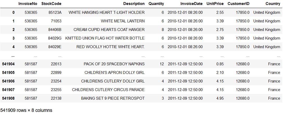
4 Data pre-processing
'''
Create an indicator column stipulating whether the invoice number begins with 'C'
'''

df['Is_C_Present'] = (
    online['InvoiceNo']
    .astype(str)
    .apply(lambda x: 1 if x.find('C') != -1 else 0))

df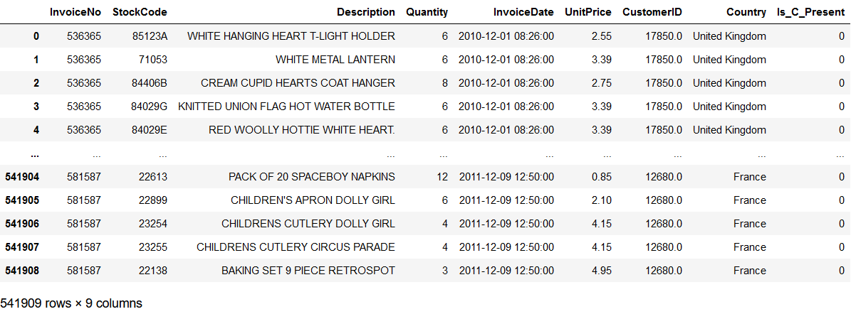
'''
Filter out all transactions having either zero or a negative number of items.
Remove all invoice numbers starting with 'C' (using columns 'Is_C_Present').
Subset the dataframe down to 'InvoiceNo' and 'Descritpion'.
Drop all rows with at least one missing value.
'''


df_clean = (
    df
    # filter out non-positive quantity values
    .loc[df["Quantity"] > 0]
    # remove InvoiceNos starting with C
    .loc[df['Is_C_Present'] != 1]
    # column filtering
    .loc[:, ["InvoiceNo", "Description"]]
    # dropping all rows with at least one missing value
    .dropna()
)

df_clean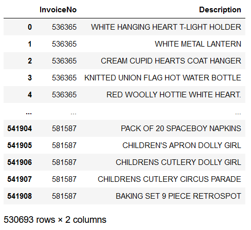
print(
    "Data dimension (row count, col count): {dim}"
    .format(dim=df_clean.shape)
)
print(
    "Count of unique invoice numbers: {cnt}"
    .format(cnt=df_clean.InvoiceNo.nunique())
)
'''
Transform the data into a list of lists called invoice_item_list

'''

invoice_item_list = []
for num in list(set(df_clean.InvoiceNo.tolist())):
    # filter data set down to one invoice number
    tmp_df = df_clean.loc[df_clean['InvoiceNo'] == num]
    # extract item descriptions and convert to list
    tmp_items = tmp_df.Description.tolist()
    # append list invoice_item_list
    invoice_item_list.append(tmp_items)

print(invoice_item_list[1:3])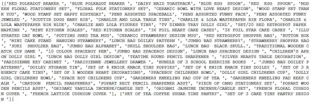
To be able to run any models the data, currently in the list of lists form, needs to be encoded and recast as a dataframe. Outputted from the encoder is a multidimensional array, where each row is the length of the total number of unique items in the transaction dataset and the elements are Boolean variables, indicating whether that particular item is linked to the invoice number that row presents. With the data encoded, we can recast it as a dataframe where the rows are the invoice numbers and the columns are the unique items in the transaction dataset.
# Initialize and fit the transaction encoder
online_encoder = mlxtend.preprocessing.TransactionEncoder()
online_encoder_array = online_encoder.fit_transform(invoice_item_list)

# Recast the encoded array as a dataframe
online_encoder_df = pd.DataFrame(online_encoder_array, columns=online_encoder.columns_)

# Print the results
online_encoder_df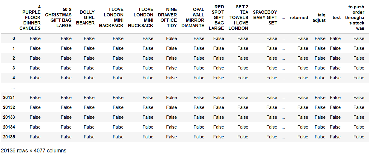
5 Executing the Apriori Algorithm
The Apriori algorithm is one of the most common techniques in Market Basket Analysis.
It is used to analyze the frequent itemsets in a transactional database, which then is used to generate association rules between the products.
'''
Run the Apriori Algorithm with min_support = 0.01 (by default 0.5)
'''

apriori_model = mlxtend.frequent_patterns.apriori(online_encoder_df, min_support=0.01)
apriori_model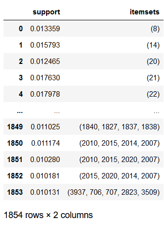
'''
Run the same model again, but this time with use_colnames=True.
This will replace the numerical designations with the actual item names.
'''

apriori_model_colnames = mlxtend.frequent_patterns.apriori(
    online_encoder_df,
    min_support=0.01,
    use_colnames=True
)

apriori_model_colnames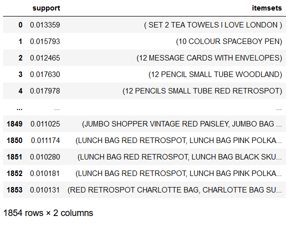
'''
Add an additional column to the output of apriori_model_colnames that contains the size of the item set.
This will help with filtering and further analysis.
'''

apriori_model_colnames['length'] = (
    apriori_model_colnames['itemsets'].apply(lambda x: len(x))
)

apriori_model_colnames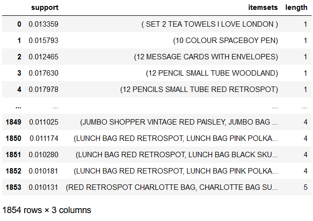
apriori_model_colnames[
    apriori_model_colnames['itemsets'] == frozenset(
        {'12 PENCIL SMALL TUBE WOODLAND'})]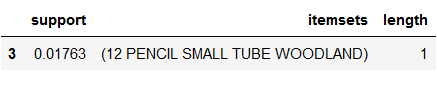
The output gives us the support value for ‘12 PENCIL SMALL TUBE WOODLAND’. The support value says that this specific item appears in 1,76% of the transactions.
apriori_model_colnames[
    (apriori_model_colnames['length'] == 2) &
    (apriori_model_colnames['support'] >= 0.02) &
    (apriori_model_colnames['support'] < 0.021)
]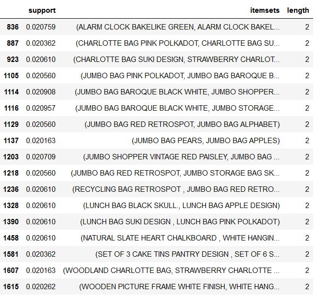
This dataframe contains all the item sets (pairs of items bought together) whose support value is in the range between 2% and 2.1% of transactions.
When you are filtering on support, it is wise to specify a range instead of a sprecific value since it is quite possible to pick a value for which there are no item sets.
apriori_model_colnames.hist("support", grid=False, bins=30)
plt.title("Support")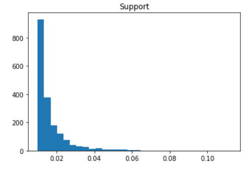
6 Deriving Association Rules
'''
Generate derive association rules for the online retail dataset.
Here we use confidence as the measure of interestingness.
Set the minimum threshold to 0.6.
Return all metrics, not just support.
'''

rules = mlxtend.frequent_patterns.association_rules(
    apriori_model_colnames,
    metric="confidence",
    min_threshold=0.6,
    support_only=False
)

rules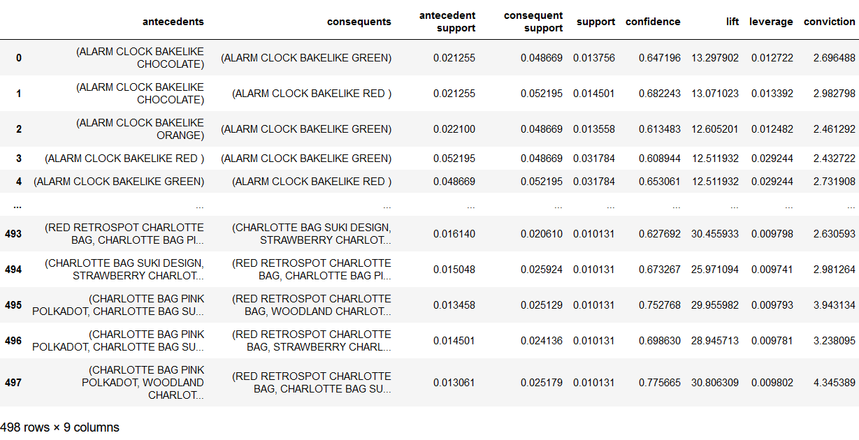
print("Number of Associations: {}".format(rules.shape[0]))
rules.plot.scatter("support", "confidence", alpha=0.5, marker="*")
plt.xlabel("Support")
plt.ylabel("Confidence")
plt.title("Association Rules")
plt.show()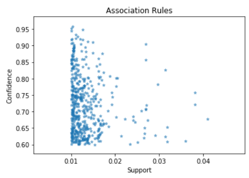
There are not any association rules with both extremly high confidence and extremely high support.
This make sense. If an item set has high support, the items are likely to appear with many other items, making the chances of high confidence very low.
7 Conclusion
In this publication I have written about what market basket analysis is and how to perform it.
With this kind of analysis from the field of mareting you can now determine which products are most often bought in combination with each other. With this knowledge it is possible to arrange the products efficiently in the store. In the best case, products that are often bought together are positioned in the opposite direction in the store so that customers are forced to walk past as many other products as possible.
Furthermore, one can now consider targeted discount campaigns. If you discount a product that is often bought in combination with others, you increase the chance of buying these products in combination, whereby a small discount is granted on only one.
References
The content of the entire post was created using the following sources:
Hwang, Y. (2019). Hands-On Data Science for Marketing: Improve your marketing strategies with machine learning using Python and R. Packt Publishing Ltd.