1 Introduction
After having reported very detailed in numerous posts about the different machine learning areas I will now work on various analytics fields.
I start with Marketing Analytics.
To be precise, the analysis of conversion rates, their influencing factors and how machine learning algorithms can be used to generate valuable insights from this kind of data.
In this post I will use the data set ‘bank-additional-full’ and ‘WA_Fn-UseC_-Marketing-Customer-Value-Analysis’. Both are from the website “UCI Machine Learning Repository”. You can also download them from my “GitHub Repository”.
2 Import the libraries
import pandas as pd
import numpy as np

import matplotlib.pyplot as plt

from sklearn.preprocessing import LabelBinarizer
from sklearn.preprocessing import OneHotEncoder

import statsmodels.api as sm

from sklearn.model_selection import train_test_split
from sklearn.ensemble import RandomForestClassifier
from sklearn.metrics import accuracy_score
from sklearn.metrics import roc_curve, auc

from sklearn.tree import DecisionTreeClassifier
from sklearn.tree import plot_tree
3 Descriptive Analytics (Conversion Rate)
Definition Conversion Rate:
The conversion rate describes the ratio of visits/clicks to conversions achieved. Conversions are conversions from prospects to customers or buyers. They can for example consist of purchases or downloads.
df = pd.read_csv('bank-additional-full.csv', sep=';')
df.head()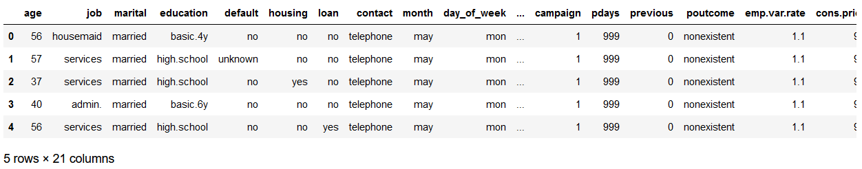
'''
In the following the column y is coded.
Then the newly generated values are inserted into the original dataframe.
The old column is still retained in this case.
'''

encoder_y = LabelBinarizer()

# Application of the LabelBinarizer
y_encoded = encoder_y.fit_transform(df.y.values.reshape(-1,1))

# Insertion of the coded values into the original data set
df['conversion'] = y_encoded

# Getting the exact coding and show new dataframe
print(encoder_y.classes_)
print('Codierung: no=0, yes=1')
print('-----------------------------')
print()
print('New Data Frame:')
df.head()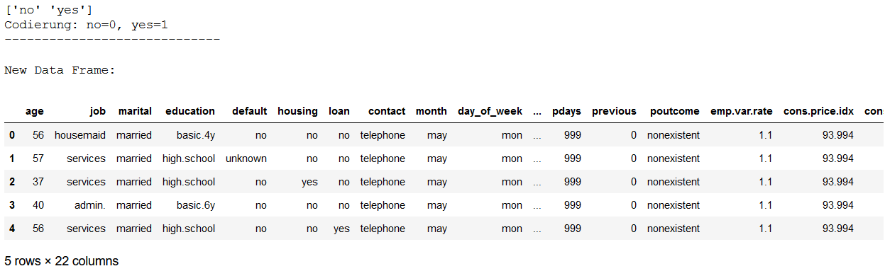
'''
Absolut conversions vs. conversion rate
'''

print('Conversions (absolut): %i out of %i' % (df.conversion.sum(), df.shape[0]))

print('Conversion Rate: %0.2f%%' % (df.conversion.sum() / df.shape[0] * 100.0))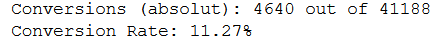
Age
'''
Calculate the conversion rate by age
'''

conversion_rate_by_age = df.groupby(by='age')['conversion'].sum() / df.groupby(by='age')['conversion'].count() * 100.0
pd.DataFrame(conversion_rate_by_age.reset_index().rename(columns={'conversion':'conversion_%'})).head()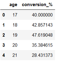
ax = conversion_rate_by_age.plot(
    grid=True,
    figsize=(10, 7),
    title='Conversion Rates by Age')

ax.set_xlabel('age')
ax.set_ylabel('conversion rate (%)')

plt.show()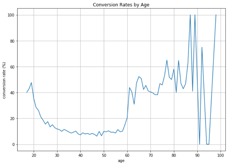
def age_group_function(df):

    if (df['age'] >= 70):
        return '70<'

    elif (df['age'] < 70) and (df['age'] >= 60):
        return '[60, 70]'

    elif (df['age'] <= 60) and (df['age'] >= 50):
        return '[50, 60]'

    elif (df['age'] <= 50) and (df['age'] >= 40):
        return '[40, 50]'

    elif (df['age'] <= 40) and (df['age'] >= 30):
        return '[30, 40]'

    elif (df['age'] <= 30) and (df['age'] >= 20):
        return '[20, 30]'

    elif (df['age'] < 20):
        return '<20'

df['age_group'] = df.apply(age_group_function, axis = 1)
df.head()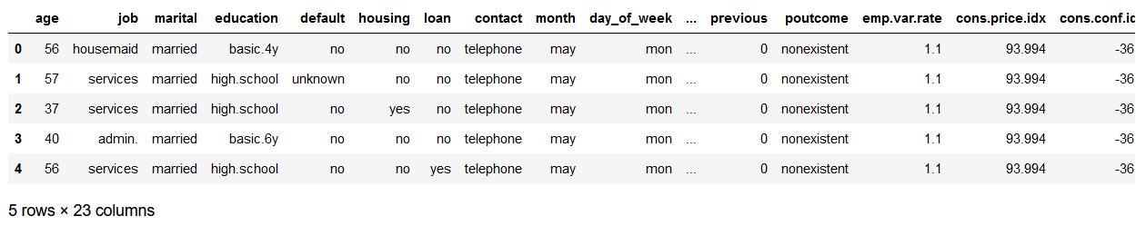
'''
Calculate the conversion rate by age_group
'''

conversion_rate_by_age_group = df.groupby(by='age_group')['conversion'].sum() / df.groupby(by='age_group')['conversion'].count() * 100.0
pd.DataFrame(conversion_rate_by_age_group.reset_index().rename(columns={'conversion':'conversion_%'}))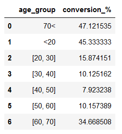
ax = conversion_rate_by_age_group.loc[['<20', '[20, 30]', '[30, 40]', '[40, 50]', '[50, 60]', '[60, 70]', '70<']].plot(
    kind='bar',
    color='skyblue',
    grid=True,
    figsize=(10, 7),
    title='Conversion Rates by Age Groups')

ax.set_xlabel('age_group')
ax.set_ylabel('conversion rate (%)')

plt.show()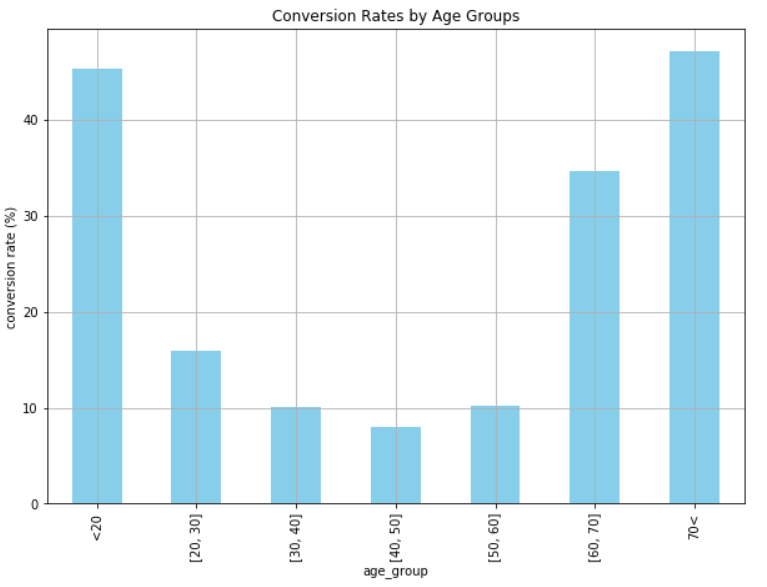
Marital Status
conversions_by_marital_status = pd.pivot_table(df, values='y', index='marital', columns='conversion', aggfunc=len)
conversions_by_marital_status.columns = ['non_conversions', 'conversions']
conversions_by_marital_status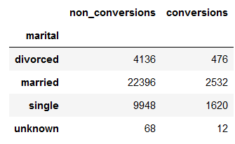
conversions_by_marital_status.plot(
    kind='pie',
    figsize=(15, 7),
    startangle=90,
    subplots=True,
    autopct=lambda x: '%0.1f%%' % x)

plt.show()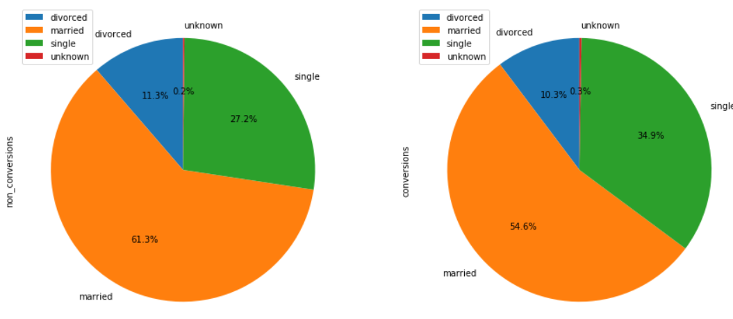
Age Groups and Marital Status
age_marital = df.groupby(['age_group', 'marital'])['conversion'].sum().unstack('marital').fillna(0)
age_marital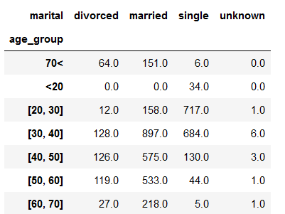
age_marital = age_marital.divide(
    df.groupby(
    by='age_group'
    )['conversion'].count(),
    axis=0)

age_marital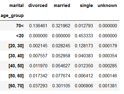
ax = age_marital.loc[
    ['<20', '[20, 30]', '[30, 40]', '[40, 50]', '[50, 60]', '[60, 70]', '70<']].plot(
    kind='bar',
    stacked=True,
    grid=True,
    figsize=(10,7))

ax.set_title('Conversion rates by Age & Marital Status')
ax.set_xlabel('age group')
ax.set_ylabel('conversion rate (%)')

plt.show()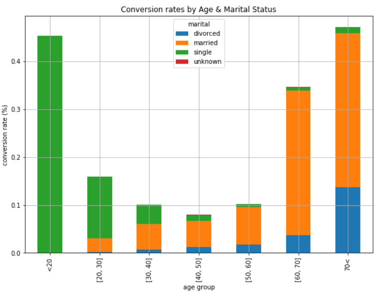
4 Drivers behind Marketing Engagement
Definiton Marketing Engagement:
In marketing engagement, the aim is to involve the customer in the marketing measures and thus encourage him to actively interact with the content. This should generate a positive experience and a positive association with the brand and the company, thus strengthening the customer’s loyalty to the company. This can lead to identification with the company and its values and can ultimately increase the chance of conversions.
df = pd.read_csv('WA_Fn-UseC_-Marketing-Customer-Value-Analysis.csv')
df['Engaged'] = df['Response'].apply(lambda x: 0 if x == 'No' else 1)
df.head().T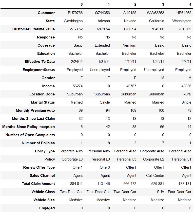
4.1 Select Numerical Columns
num_col = ['int16', 'int32', 'int64', 'float16', 'float32', 'float64']
numerical_columns = list(df.select_dtypes(include=num_col).columns)
df_numeric = df[numerical_columns]
df_numeric.dtypes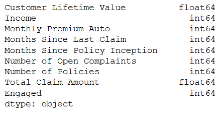
4.2 Select and Encode Categorical Columns
obj_col = ['object']
object_columns = list(df.select_dtypes(include=obj_col).columns)
df_categorical = df[object_columns]
df_categorical.dtypes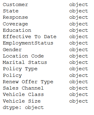
We just take 3 of the cat variables otherwise this step would take too long and this is just an example of how to handle cat variables.
df_categorical = df_categorical[['State', 'Education', 'Gender']]
df_categorical.head()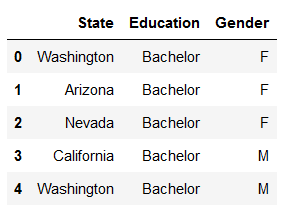
print('Values of the variable State:')
print()
print(df_categorical['State'].value_counts())

print('--------------------------------------------')

print('Values of the variable Education:')
print()
print(df_categorical['Education'].value_counts())

print('--------------------------------------------')

print('Values of the variable EmploymentStatus:')
print()
print(df_categorical['Gender'].value_counts())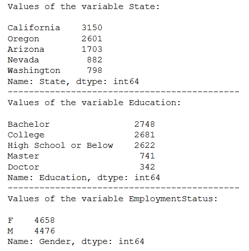
Here we have 3 different kind of categorical variables.
- State: nominal
- Education: ordinal
- Gender: binary
In the following the column State is coded. Then the newly generated values are inserted into the original dataframe and the old column will be deleted.
encoder_State = OneHotEncoder()

# Application of the OneHotEncoder
OHE = encoder_State.fit_transform(df_categorical.State.values.reshape(-1,1)).toarray()

# Conversion of the newly generated data to a dataframe
df_OHE = pd.DataFrame(OHE, columns = ["State_" + str(encoder_State.categories_[0][i])
                                     for i in range(len(encoder_State.categories_[0]))])


# Insertion of the coded values into the original data set
df_categorical = pd.concat([df_categorical, df_OHE], axis=1)


# Delete the original column to avoid duplication
df_categorical = df_categorical.drop(['State'], axis=1)
In the following the column Education is coded. Then the newly generated values are inserted into the original dataframe and the old column will be deleted.
# Create a dictionary how the observations should be coded
education_dict = {'High School or Below' : 0,
                  'College' : 1,
                  'Bachelor' : 2,
                  'Master' : 3,
                  'Doctor' : 4}

# Map the dictionary on the column view and store the results in a new column
df_categorical['Education_encoded'] = df_categorical.Education.map(education_dict)

# Delete the original column to avoid duplication
df_categorical = df_categorical.drop(['Education'], axis=1)
In the following the column Gender is coded. Then the newly generated values are inserted into the original dataframe and the old column will be deleted.
encoder_Gender = LabelBinarizer()

# Application of the LabelBinarizer
Gender_encoded = encoder_Gender.fit_transform(df_categorical.Gender.values.reshape(-1,1))

# Insertion of the coded values into the original data set
df_categorical['Gender_encoded'] = Gender_encoded

# Delete the original column to avoid duplication
df_categorical = df_categorical.drop(['Gender'], axis=1)
4.3 Create final Dataframe
df_final = pd.concat([df_numeric, df_categorical], axis=1)
df_final.head()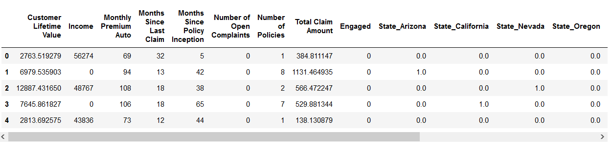
4.4 Regression Analysis (Logit)
If we work with the sm library, we have to add a constant to the predictor(s). With the Statsmodels Formula library, this would not have been necessary manually, but the disadvantage of this variant is that we have to enumerate the predictors individually in the formula.
x = sm.add_constant(df_final.drop('Engaged', axis=1))

y = df_final['Engaged']
logit = sm.Logit(y,x)
logit_fit = logit.fit()
logit_fit.summary()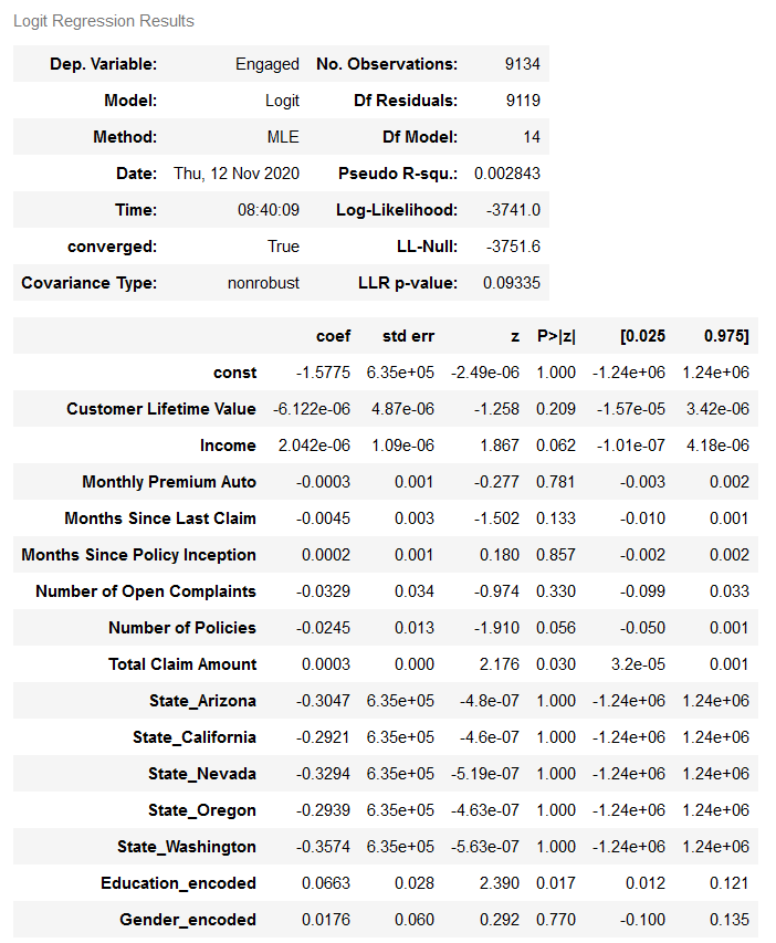
2 variables are significant (Education_encoded and Total Claim Amount). Both with a positive relationship to the target variable Engaged.
This means (in the case of the variable Education_encoded), the higher the education the more the customer will be receptive to marketing calls.
5 Predicting the Likelihood of Marketing Engagement
Here we can again use the previously created data set (df_final). Note at this point: We have not included all categorical variables. The reason for this was that the correct coding was not done for all variables for reasons of overview/time.
# Replacement of all whitespaces within the column names
df_final.columns = [x.replace(' ', '_') for x in df_final.columns]
df_final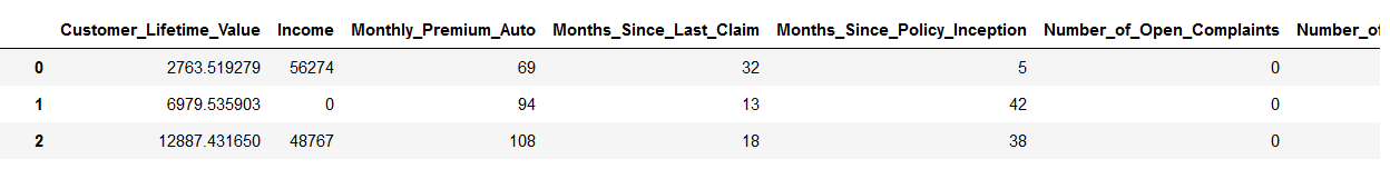
x = df_final.drop(['Engaged'], axis=1)
y = df_final['Engaged']

trainX, testX, trainY, testY = train_test_split(x, y, test_size = 0.2)
5.1 Fit the Model
rf_model = RandomForestClassifier(n_estimators=200, max_depth=5)
rf_model.fit(trainX, trainY)
5.2 Feature Importance
feat_imps = pd.DataFrame({'importance': rf_model.feature_importances_}, index=trainX.columns)
feat_imps.sort_values(by='importance', ascending=False, inplace=True)
feat_imps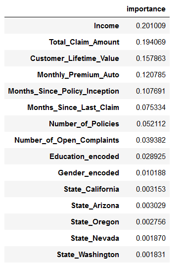
feat_imps.plot(kind='bar', figsize=(10,7))

plt.legend()
plt.show()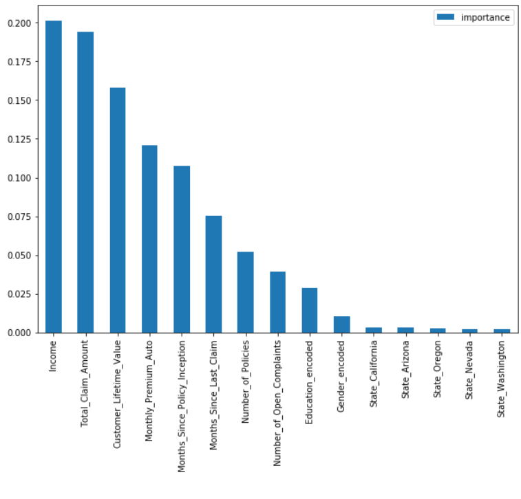
5.3 Model Evaluation
Accuracy
rf_preds_train = rf_model.predict(trainX)
rf_preds_test = rf_model.predict(testX)

print('Random Forest Classifier:\n> Accuracy on training data = {:.4f}\n> Accuracy on test data = {:.4f}'.format(
    accuracy_score(trainY, rf_preds_train),
    accuracy_score(testY, rf_preds_test)
))
ROC & AUC
rf_preds_train = rf_model.predict_proba(trainX)[:,1]
rf_preds_test = rf_model.predict_proba(testX)[:,1]
train_fpr, train_tpr, train_thresholds = roc_curve(trainY, rf_preds_train)
test_fpr, test_tpr, test_thresholds = roc_curve(testY, rf_preds_test)train_roc_auc = auc(train_fpr, train_tpr)
test_roc_auc = auc(test_fpr, test_tpr)
print('Train AUC: %0.4f' % train_roc_auc)
print('Test AUC: %0.4f' % test_roc_auc)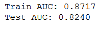
plt.figure(figsize=(10,7))

plt.plot(test_fpr, test_tpr, color='darkorange', label='Test ROC curve (area = %0.4f)' % test_roc_auc)
plt.plot(train_fpr, train_tpr, color='navy', label='Train ROC curve (area = %0.4f)' % train_roc_auc)
plt.plot([0, 1], [0, 1], color='gray', lw=1, linestyle='--')
plt.grid()
plt.xlim([0.0, 1.0])
plt.ylim([0.0, 1.05])
plt.xlabel('False Positive Rate')
plt.ylabel('True Positive Rate')
plt.title('RandomForest Model ROC Curve')
plt.legend(loc="lower right")

plt.show()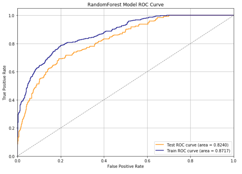
6 Engagement to Conversion
Now that we have examined the conversion rate by means of descriptive statistics, have determined the influencing factors of engagement and can also predict these by means of a machine learning model, it is now time to extract further insights, such as a target group determination, from the data to the conversion rate.
df = pd.read_csv('bank-additional-full.csv', sep=';')
df.head()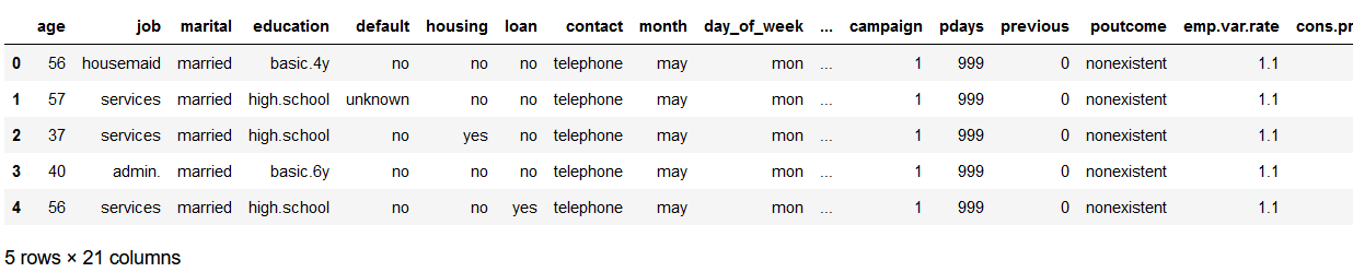
num_col = ['int16', 'int32', 'int64', 'float16', 'float32', 'float64']
numerical_columns = list(df.select_dtypes(include=num_col).columns)
df_numeric = df[numerical_columns]
df_numeric = df_numeric[['age', 'campaign']]
df_numeric.dtypes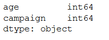
obj_col = ['object']
object_columns = list(df.select_dtypes(include=obj_col).columns)
df_categorical = df[object_columns]
df_categorical = df_categorical[['job', 'marital', 'y']]
df_categorical.dtypes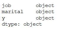
dummy_job = pd.get_dummies(df_categorical['job'], prefix="job")
column_name = df_categorical.columns.values.tolist()
column_name.remove('job')
df_categorical = df_categorical[column_name].join(dummy_job)

dummy_marital = pd.get_dummies(df_categorical['marital'], prefix="marital")
column_name = df_categorical.columns.values.tolist()
column_name.remove('marital')
df_categorical = df_categorical[column_name].join(dummy_marital)


df_categorical.head()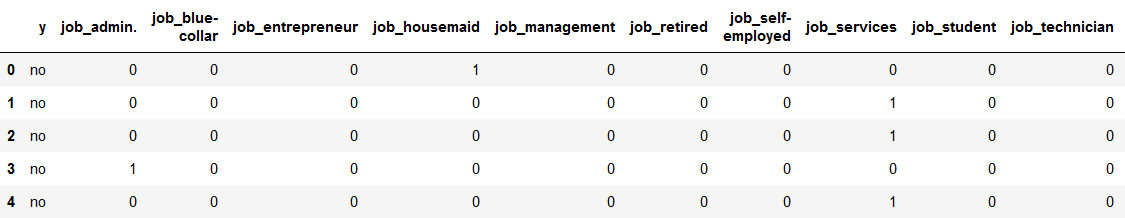
df_final = pd.concat([df_categorical, df_numeric], axis=1)
df_final.head()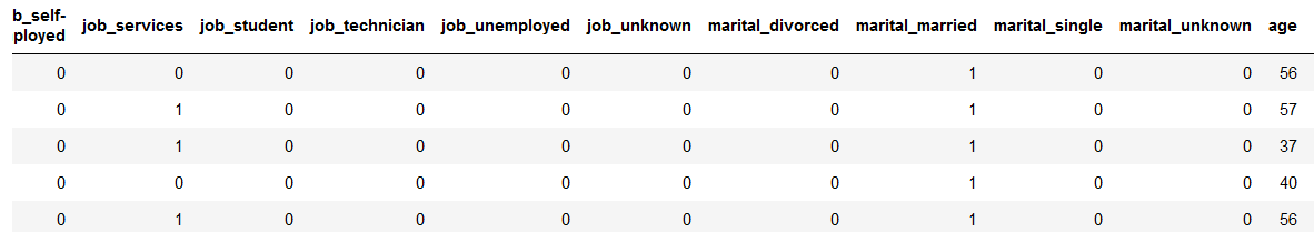
x = df_final.drop(['y'], axis=1)
y = df_final['y']
clf_dt = DecisionTreeClassifier()
clf_dt.fit(x, y)features = x.columns.tolist()
classes = y.unique().tolist()
plt.figure(figsize=(15, 15))
plot_tree(clf_dt, feature_names=features, class_names=classes, filled=True)
plt.savefig('tree.png')
plt.show()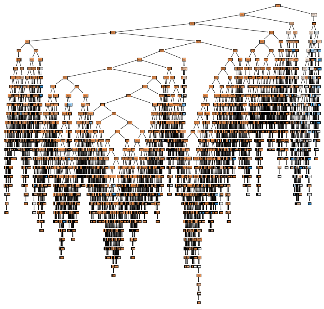
Not yet really readable / interpretable.
clf = DecisionTreeClassifier(max_depth=4)
clf.fit(x, y)
features = x.columns.tolist()
classes = y.unique().tolist()
plt.figure(figsize=(150, 150))
plot_tree(clf, feature_names=features, class_names=classes, filled=True)
plt.savefig('tree2.png')
plt.show()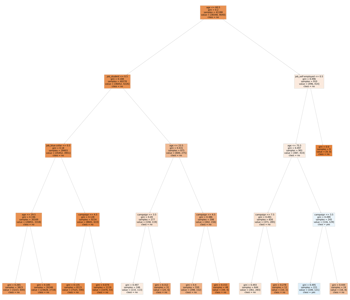
Already much better. I personally always save the generated chart separately to be able to view the results in more detail if necessary.
Those customers that belong to the eleventh leaf node from the left are those with a 0 value for the self_employed variable, age greater than 75.5 and a campaign variable with a value of less than 3.5.
In other words, those who are not self employed, older than 75.5 and have come in contact with the campaigns 1-3 have a high chance of converting.
7 Conclusion
The following points were covered in the main chapters 3-6:
- Descriptive Analysis at Conversion Rate.
- Determine reasons for Marketing Engagement.
- Prediction of marketing engagement.
- Determination and analysis of the target group that causes conversions.
References
The content of the entire post was created using the following sources:
Hwang, Y. (2019). Hands-On Data Science for Marketing: Improve your marketing strategies with machine learning using Python and R. Packt Publishing Ltd.