1 Introduction
K Nearest Neighbor (KNN) is a very simple supervised classification algorithm which is easy to understand, versatile and one of the topmost machine learning algorithms. The KNN algorithm can be used for both classification (binary and multiple) and regression problems.
For this post the dataset Iris from the statistic platform “Kaggle” was used. You can download it from my “GitHub Repository”.
2 Background information on KNN
In general we can say KNN is a non-parametric and lazy learning algorithm.
Non-parametric means there is no assumption for underlying data distribution. But this will be very helpful in practice where most of the real world datasets do not follow mathematical theoretical assumptions.
Lazy Learning means there is no need for learning or training of the model and all of the data points used at the time of prediction. Lazy learners wait until the last minute before classifying any data point. In comparison to that eager learners will construct with given training points a generalized model before performing prediction on given new points to classify.
Curse of Dimensionality
K Nearest Neighbor performs better with a lower number of features than a large number of features. You can say that when the number of features increases than it requires much more data. Increase in dimension also leads to the problem of overfitting. To avoid overfitting, the needed data will need to grow exponentially as you increase the number of dimensions. This problem of higher dimension is known as the Curse of Dimensionality.
How does the KNN algorithm work?
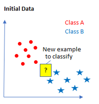
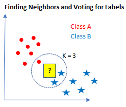
In KNN, K is the number of nearest neighbors. KNN works as described in the following steps:
- Computes the distance between the new data point with every training example.
- For computing the distance measures such as Euclidean distance, Manhattan or Hamming distance will be used.
- Model picks K entries in the database which are closest to the new data point.
- Then it does the majority vote i.e the most common class/label among those K entries will be the class of the new data point.
I have shown the individual steps visually below:


Pros:
- The training phase of K-nearest neighbor classification is much faster compared to other classification algorithms.
- There is no need to train a model for generalization, That is why KNN is known as the simple and instance-based learning algorithm.
- KNN can be useful in case of nonlinear data.
- It can be used with the regression problem. Output value for the object is computed by the average of k closest neighbors value.
Cons:
- The testing phase of K-nearest neighbor classification is slower and costlier in terms of time and memory.
- It requires large memory for storing the entire training dataset for prediction.
- Euclidean distance is sensitive to magnitudes.
- The features with high magnitudes will weight more than features with low magnitudes.
- KNN also not suitable for large dimensional data.
3 Loading the libraries and the data
import numpy as np
import pandas as pd

from sklearn.model_selection import train_test_split

from sklearn.neighbors import KNeighborsClassifier
from sklearn.metrics import accuracy_score

from sklearn.model_selection import cross_val_score

%matplotlib inline
import matplotlib.pyplot as plt

from sklearn.model_selection import GridSearchCV
iris = pd.read_csv("path/to/file/Iris_Data.csv")
iris
4 KNN - Model Fitting and Evaluation
As always, we split the data set into a training and a test part.
x = iris.drop('species', axis=1)
y = iris['species']

trainX, testX, trainY, testY = train_test_split(x, y, test_size = 0.2)
With the parameter n_neighbors we determine the number of K. Here we just set K to 7 and look at the accuracy rate.
knn_clf = KNeighborsClassifier(n_neighbors=7)

knn_clf.fit(trainX, trainY)

y_pred = knn_clf.predict(testX)

print('Accuracy: {:.2f}'.format(accuracy_score(testY, y_pred)))
Ok, accuracy rate of .90. Not so bad. Let’s evaluate our model with cross validation technique.
knn_clf = KNeighborsClassifier(n_neighbors=5)

scores = cross_val_score(knn_clf, trainX, trainY, cv=10, scoring='accuracy')
print(scores)
As we can see, there is still room for improvement.
5 Determination of K and Model Improvement
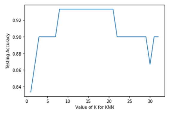
With the following for loop we have the respective accuracy rate output for different K’s (here K:1-33).
k_range = range(1, 33)
scores = {}
scores_list = []

for k in k_range:
    knn = KNeighborsClassifier(n_neighbors=k)
    knn.fit(trainX, trainY)
    y_pred = knn.predict(testX)
    scores[k] = accuracy_score(testY, y_pred)
    scores_list.append(accuracy_score(testY, y_pred))
Let’s plot the results:
plt.plot(k_range, scores_list)
plt.xlabel('Value of K for KNN')
plt.ylabel('Testing Accuracy')
As we can see, K = 7 was probably set a little too low in the first model. It seems that we get the best accuracy value for K = 8. Let’s check this with Grid Search.
k_range = list(range(1,33))
weight_options = ["uniform", "distance"]

knn_clf = KNeighborsClassifier()
param_grid = dict(n_neighbors=k_range, weights=weight_options)

grid = GridSearchCV(knn_clf, param_grid, cv=10, scoring='accuracy')
grid.fit(trainX, trainY)
print(grid.best_params_)
We were right with our assumption. Let’s set K to 8.
knn_clf = KNeighborsClassifier(n_neighbors=8, weights='distance')

knn_clf.fit(trainX, trainY)

y_pred = knn_clf.predict(testX)

print('Accuracy: {:.2f}'.format(accuracy_score(testY, y_pred)))
We can also use the trained grid model right away, as this saved the best values.
grid_predictions = grid.predict(testX)

print('Accuracy: {:.2f}'.format(accuracy_score(testY, grid_predictions)))
6 Conclusion
This publication explains what the K Nearest Neighbor Classifier is and how we can use it to solve classification problems. Furthermore, the determination of K was discussed.