1 Introduction
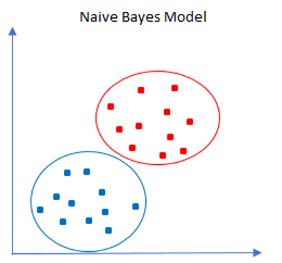
Now in the series of multiple classifiers we come to a very easy to use probability model: The Naive Bayes Classifier.
Due to the fact that this algorithm has hardly any hyperparameters, it is recommended to always use the Naive Bayes Classifier first in the event of classification problems. If this does not give satisfactory results, however, more complex algorithms should be used.
For this post the dataset Wine Quality from the statistic platform “Kaggle” was used. You can download it from my “GitHub Repository”.
2 Background information on Naive Bayes Classifier
Naive Bayes classifiers
One of the simplest yet effective algorithm that should be tried to solve the classification problem is Naive Bayes Algorithm. It’s a probabilistic modell which is based on the Bayes’ theorem which is an equation describing the relationship of conditional probabilities of statistical quantities.
Naive Bayes in scikit-learn
The scikit-learn library includes three naive Bayes variants based on the same number of different probabilistic distributions: Gaussian, Multinomial and Bernoulli
Gaussian Naive Bayes
Perhaps the easiest naive Bayes classifier to understand is Gaussian naive Bayes Classifier. When the predictors take up a continuous value and are not discrete, we assume that these values are sampled from a gaussian distribution.
Multinomial Naive Bayes
The assumption about Gaussian just described is by no means the only simple assumption that could be used to specify the generative distribution for each label. Another very useful example is multinomial naive Bayes, where the features are assumed to be generated from a simple multinomial distribution. The multinomial distribution describes the probability of observing counts among a number of categories, and thus multinomial naive Bayes is most appropriate for features that represent counts or count rates. The idea is precisely the same as before, except that instead of modeling the data distribution with the best-fit Gaussian, we model the data distribuiton with a best-fit multinomial distribution.
Bernoulli Naive Bayes
This is similar to the multinomial naive bayes but the predictors are boolean variables. The parameters that we use to predict the class variable take up only values Yes or No.
Pros and Cons of Naive Bayes
Pros:
- It is not only a simple approach but also a fast and accurate method for prediction.
- Naive Bayes has very low computation cost.
- It is easy and fast to predict class of test data set. It also perform well in multi class prediction
- When assumption of independence holds, a Naive Bayes classifier performs better compare to other models like logistic regression and you need less training data.
- It performs well in case of discrete response variable compared to the continuous variable.
- It also performs well in the case of text analytics problems.
- When the assumption of independence holds, a Naive Bayes classifier performs better compared to other models like logistic regression.
Cons:
- If categorical variable has a category in test data set, which was not observed in training data set, then model will assign a zero probability and will be unable to make a prediction. This is often known as “Zero Frequency”.
- Naive Bayes is also known as a bad estimator, so the probability outputs from predict_proba are not to be taken too seriously.
- Another limitation of Naive Bayes is the assumption of independent predictors. In real life, it is almost impossible that we get a set of predictors which are completely independent.
3 Loading the libraries and the data
import numpy as np
import pandas as pd

# For Chapter 4
from sklearn.preprocessing import LabelBinarizer

# For Chapter 5
from sklearn.model_selection import train_test_split
from sklearn.metrics import accuracy_score
from sklearn.metrics import confusion_matrix

from sklearn.naive_bayes import GaussianNB
from sklearn.naive_bayes import BernoulliNB
from sklearn.naive_bayes import MultinomialNB
wine = pd.read_csv("path/to/file/winequality.csv")
wine.head()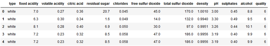
4 Data pre-processing
Let’s have a glimpse at the variable ‘type’:
wine['type'].value_counts().T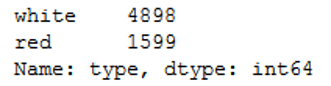
The division between white wine and red wine is not quite equal in this data set. Let’s encode this variable for further processing.
encoder = LabelBinarizer()
encoded_type = encoder.fit_transform(wine.type.values.reshape(-1,1))

wine['encoded_type'] = encoded_type
wine['encoded_type'] = wine['encoded_type'].astype('int64')
wine = wine.drop('type', axis=1)
wine.head()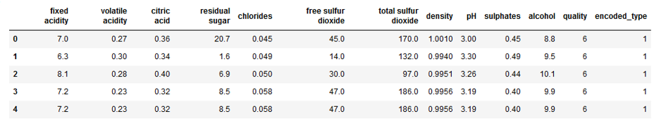
Now we check for missing values:
def missing_values_table(df):
        # Total missing values
        mis_val = df.isnull().sum()

        # Percentage of missing values
        mis_val_percent = 100 * df.isnull().sum() / len(df)

        # Make a table with the results
        mis_val_table = pd.concat([mis_val, mis_val_percent], axis=1)

        # Rename the columns
        mis_val_table_ren_columns = mis_val_table.rename(
        columns = {0 : 'Missing Values', 1 : '% of Total Values'})

        # Sort the table by percentage of missing descending
        mis_val_table_ren_columns = mis_val_table_ren_columns[
            mis_val_table_ren_columns.iloc[:,1] != 0].sort_values(
        '% of Total Values', ascending=False).round(1)

        # Print some summary information
        print ("Your selected dataframe has " + str(df.shape[1]) + " columns.\n"
            "There are " + str(mis_val_table_ren_columns.shape[0]) +
              " columns that have missing values.")

        # Return the dataframe with missing information
        return mis_val_table_ren_columns

missing_values_table(wine)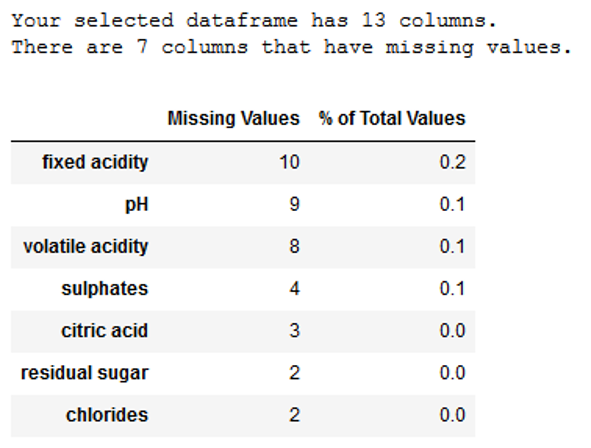
As we can see, there are a couple of missing values. Let’s remove them.
wine = wine.dropna()Let’s have a further glimpse at the variable ‘quality’:
wine['quality'].value_counts().T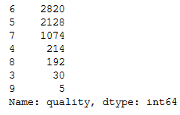
7 of 9 categories are represented. To simplify these, they are now grouped into just 3 categories (1-4, 5-7 and 8-9).
def new_quality_ranking(df):

    if (df['quality'] <= 4):
        return 1

    elif (df['quality'] > 4) and (df['quality'] < 8):
        return 2

    elif (df['quality'] <= 8):
        return 3

wine['new_quality_ranking'] = wine.apply(new_quality_ranking, axis = 1)
wine = wine.drop('quality', axis=1)
wine = wine.dropna()
wine.head()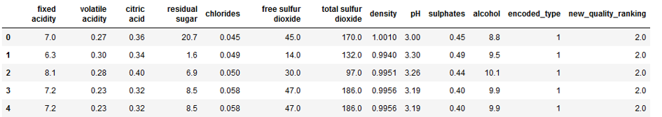
Here is the new division.
wine['new_quality_ranking'].value_counts().T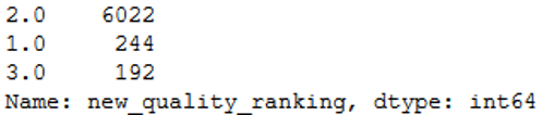
5 Naive Bayes in scikit-learn
The following shows how the naive bayes classifier types described above can be used.
5.1 Binary Classification
For the binary classification, the wine type is our target variable.
x = wine.drop('encoded_type', axis=1)
y = wine['encoded_type']
trainX, testX, trainY, testY = train_test_split(x, y, test_size = 0.2)
5.1.1 Gaussian Naive Bayes
gnb = GaussianNB()

gnb.fit(trainX, trainY)

y_pred = gnb.predict(testX)

print('Accuracy: {:.2f}'.format(accuracy_score(testY, y_pred)))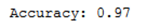
5.1.2 Bernoulli Naive Bayes
bnb = BernoulliNB(binarize=0.0)

bnb.fit(trainX, trainY)

y_pred = bnb.predict(testX)

print('Accuracy: {:.2f}'.format(accuracy_score(testY, y_pred)))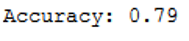
5.2 Multiple Classification
For the multiple classification, the quality ranking is our target variable.
x = wine.drop('new_quality_ranking', axis=1)
y = wine['new_quality_ranking']
trainX, testX, trainY, testY = train_test_split(x, y, test_size = 0.2)
5.2.1 Gaussian Naive Bayes
gnb = GaussianNB()

gnb.fit(trainX, trainY)

y_pred = gnb.predict(testX)

print('Accuracy: {:.2f}'.format(accuracy_score(testY, y_pred)))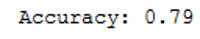
5.2.2 Multinomial Naive Bayes
mnb = MultinomialNB()

mnb.fit(trainX, trainY)

y_pred = mnb.predict(testX)

print('Accuracy: {:.2f}'.format(accuracy_score(testY, y_pred)))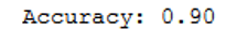
6 Conclusion
We showed in this post what Naive Bayes Classifiers are and how they can be used. Here are a few more Applications of Naive Bayes Algorithms:
- Real time Prediction: Naive Bayes is an eager learning classifier and it is sure fast. Thus, it could be used for making predictions in real time.
- Multi class Prediction: This algorithm is also well known for multi class prediction feature.
- Text classification/ Spam Filtering/ Sentiment Analysis: Naive Bayes classifiers mostly used in text classification (due to better result in multi class problems and independence rule) have higher success rate as compared to other algorithms.