1 Introduction

After “Multinomial logistic regression” we come to a further multiple class classifier: Decision Trees.
For this post the dataset Iris from the statistic platform “Kaggle” was used. You can download the dataset from my “GitHub Repository”.
2 Background information on decision trees
A decision tree is a largely used non-parametric effective machine learning modeling technique for regression and classification problems. In the following, the classification using decision trees is discussed in detail. The use of decision trees for regression problems is covered in a separate post.
Decision tree algorithms use information gain to split a node. Gini index or entropy is the criterion for calculating information gain.
Both gini and entropy are measures of impurity of a node. A node having multiple classes is impure whereas a node having only one class is pure.
Gini measurement is the probability of a random sample being classified incorrectly if we randomly pick a label according to the distribution in a branch.
Entropy is a measurement of information. You calculate the information gain by making a split.
There are several pos and cons for the use of decision trees:
Pros:
- Decision trees can be used to predict both continuous and discrete values i.e. they work well for both regression and classification tasks.
- Decision trees are easy to interpret and visualize.
- It can easily capture Non-linear patterns.
- Compared to other algorithms decision trees requires less effort for data preparation during pre-processing (e.g. no transformation of category variables necessary)
- A decision tree does not require normalization of data.
- A decision tree does not require scaling of data as well.
- Missing values in the data also does not affect the process of building decision tree to any considerable extent.
- The decision tree has no assumptions about distribution because of the non-parametric nature of the algorithm.
Cons:
- Sensitive to noisy data. It can overfit noisy data.
- A small change in the data can cause a large change in the structure of the decision tree causing instability.
- For a Decision tree sometimes calculation can go far more complex compared to other algorithms.
- Decision trees are biased with imbalance dataset, so it is recommended that balance out the dataset before creating the decision tree.
3 Loading the libraries and the data
import numpy as np
import pandas as pd


# For chapter 3
from sklearn.model_selection import train_test_split
from sklearn.tree import DecisionTreeClassifier
# For chapter 4
from sklearn.tree import export_graphviz
from pydotplus import graph_from_dot_data
import matplotlib.pyplot as plt
import matplotlib.image as img
# For chapter 5
from sklearn import metrics
from sklearn.model_selection import cross_val_score
# For chapter 6.1
from sklearn.model_selection import GridSearchCV
iris = pd.read_csv("path/to/file/Iris_Data.csv")4 Decision Trees with scikit-learn
x = iris.drop('species', axis=1)
y = iris['species']

trainX, testX, trainY, testY = train_test_split(x, y, test_size = 0.2)

clf = DecisionTreeClassifier()

clf.fit(trainX, trainY)

y_pred = clf.predict(testX)
Here we assigned the predictor variables and the target variable to an object, divided them into a training part and a test part and predicted values for the test part using the trained classification algorithm.
5 Visualization of the decision tree
5.1 via graphviz
I recommend export_graphviz for the visualization of decision trees.
class_names = y.unique().tolist()dot_data = export_graphviz(
clf,
out_file = None,
feature_names = list(trainX.columns),
class_names = str(class_names),
filled = True,
rounded = True)
graph = graph_from_dot_data(dot_data)
graph.write_png('tree.jpng')A .jpng is created and saved under the path (active directorey).
im = img.imread('tree.jpng')
plt.figure(figsize = (10,10))
plt.imshow(im)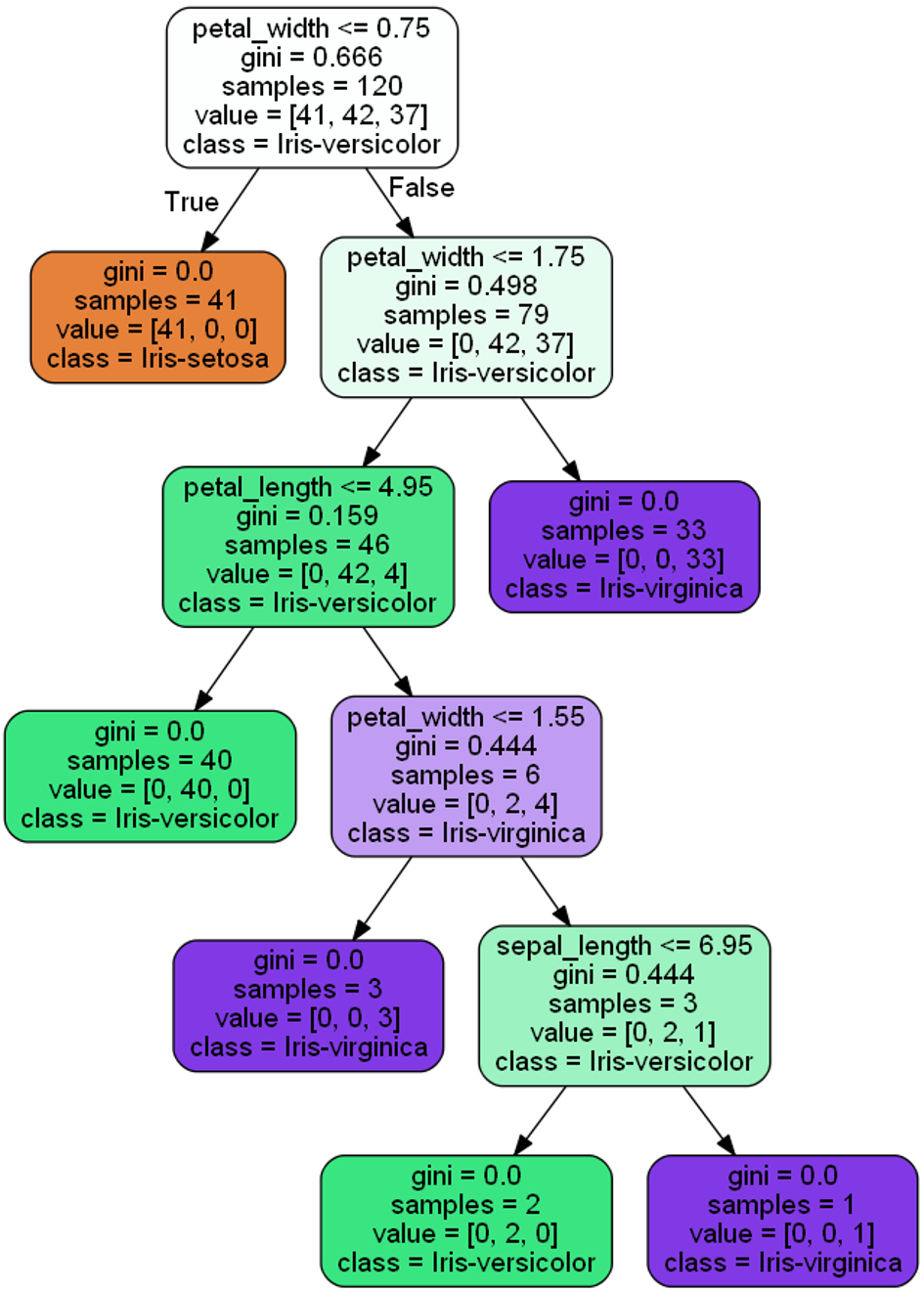
Calling the generated .jpg may show an image with poor quality. I therefore recommend calling the .jpgs directly.
5.2 via scikit-learn
New in scikit-learn (version 0.21) is plot_tree and export_text.
features = x.columns.tolist()
classes = y.unique().tolist()
plt.figure(figsize=(15, 15))
plot_tree(clf, feature_names=features, class_names=classes, filled=True)
plt.savefig('tree2.png') #you can also comment out this feature if you want
plt.show()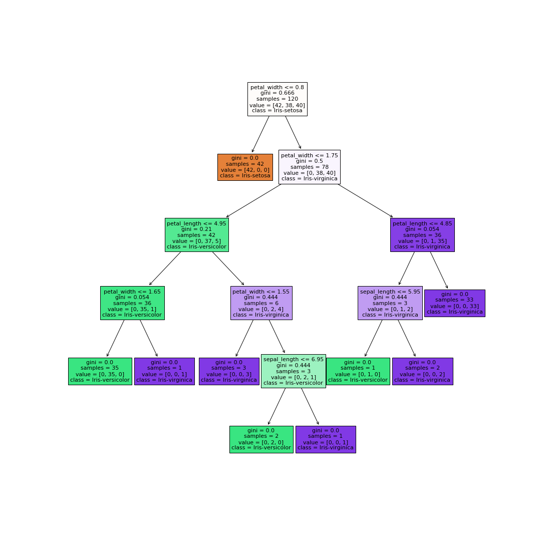
print(export_text(clf, feature_names=features, show_weights=True))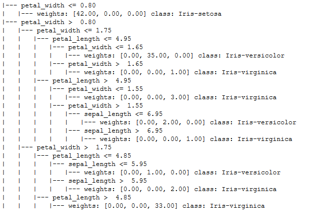
6 Model evaluation
To evaluate the model we calculate the accuracy:
metrics.accuracy_score(testY, y_pred)
Furthermore we use cross validation:
scores = cross_val_score(clf, trainX, trainY, cv=10)
print("Cross-Validation mean: {:.3f} (std: {:.3f})".format(scores.mean(),
                                          scores.std()),
                                          end="\n\n" )
Ok, here we get a slightly better result of 96.7% accuracy.
7 Model improvement
7.1 Hyperparameter optimization via Grid Search
To get a more detailed impression of how grid search works have look “here”.
param_grid = {"criterion": ["gini", "entropy"],
              "min_samples_split": [2, 5, 10, 15, 20],
              "max_depth": [None, 2, 3, 5, 7, 10],
              "min_samples_leaf": [1, 3, 5, 7, 10],
              "max_leaf_nodes": [None, 3, 5, 7, 10, 15, 20],
              }

grid = GridSearchCV(clf, param_grid, cv=10, scoring='accuracy')
grid.fit(trainX, trainY)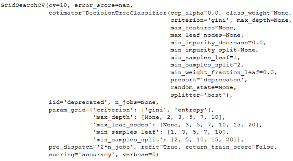
# Single best score achieved across all params
print(grid.best_score_)
# Dictionary containing the parameters used to generate that score
print(grid.best_params_)
7.2 Pruning
Another way to improve model performance is to prune a tree.
The DecisionTreeClassifier provides parameters such as min_samples_leaf and max_depth to prevent a tree from overfiting. Cost complexity pruning provides another option to control the size of a tree. In DecisionTreeClassifier, this pruning technique is parameterized by the cost complexity parameter, ccp_alpha.
path = clf.cost_complexity_pruning_path(trainX, trainY)
ccp_alphas, impurities = path.ccp_alphas, path.impurities
fig, ax = plt.subplots()
ax.plot(ccp_alphas[:-1], impurities[:-1], marker='o', drawstyle="steps-post")
ax.set_xlabel("effective alpha")
ax.set_ylabel("total impurity of leaves")
ax.set_title("Total Impurity vs effective alpha for training set")
#In the following plot, the maximum effective alpha value is removed, because it is the trivial tree with only one node.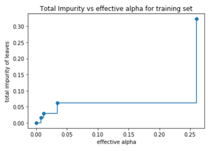
As alpha increases, more of the tree is pruned, which increases the total impurity of its leaves.
Next, we train a decision tree using the effective alphas. The last value in ccp_alphas is the alpha value that prunes the whole tree, leaving the tree, clfs[-1], with one node.
clfs = []
for ccp_alpha in ccp_alphas:
    clf = DecisionTreeClassifier(ccp_alpha=ccp_alpha)
    clf.fit(trainX, trainY)
    clfs.append(clf)
print("Number of nodes in the last tree is: {} with ccp_alpha: {}".format(
      clfs[-1].tree_.node_count, ccp_alphas[-1]))
In the following we can see that the number of nodes and tree depth decreases as alpha increases.
clfs = clfs[:-1]
ccp_alphas = ccp_alphas[:-1]

node_counts = [clf.tree_.node_count for clf in clfs]
depth = [clf.tree_.max_depth for clf in clfs]
fig, ax = plt.subplots(2, 1)
ax[0].plot(ccp_alphas, node_counts, marker='o', drawstyle="steps-post")
ax[0].set_xlabel("alpha")
ax[0].set_ylabel("number of nodes")
ax[0].set_title("Number of nodes vs alpha")
ax[1].plot(ccp_alphas, depth, marker='o', drawstyle="steps-post")
ax[1].set_xlabel("alpha")
ax[1].set_ylabel("depth of tree")
ax[1].set_title("Depth vs alpha")
fig.tight_layout()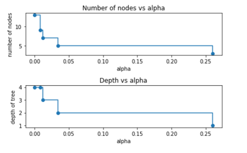
train_scores = [clf.score(trainX, trainY) for clf in clfs]
test_scores = [clf.score(testX, testY) for clf in clfs]

fig, ax = plt.subplots()
ax.set_xlabel("alpha")
ax.set_ylabel("accuracy")
ax.set_title("Accuracy vs alpha for training and testing sets")
ax.plot(ccp_alphas, train_scores, marker='o', label="train",
        drawstyle="steps-post")
ax.plot(ccp_alphas, test_scores, marker='o', label="test",
        drawstyle="steps-post")
ax.legend()
plt.show()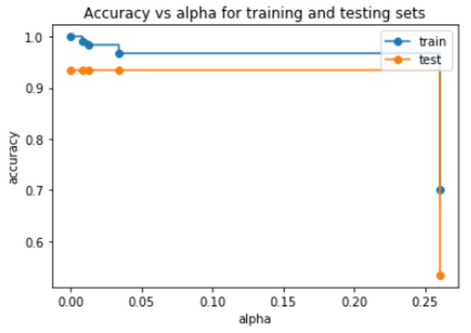
As the alpha increases, the tree becomes more pruned, creating a decision tree that may be more generalized. Here we can see that increasing ccp_alpha does not further increase accuracy
8 Conclusion
This post showed how decision trees can be created, their performance can be measured and improved. Furthermore, the advantages and disadvantages of decision trees were discussed.