1 Introduction
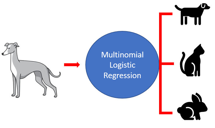
In my previous posts, I explained how “Logistic Regression” and “Support Vector Machines” works. Short wrap up: we used a logistic regression or a support vector machine to create a binary classification model. With a Multinomial Logistic Regression (also known as Softmax Regression) it is possible to predict multipe classes. And this is the content this publication is about.
For this post the dataset Iris from the statistic platform “Kaggle” was used. You can download the dataset from my “GitHub Repository”.
2 Loading the libraries and the data
import numpy as np
import pandas as pd

from sklearn.linear_model import LogisticRegression
from sklearn.model_selection import train_test_split
from sklearn import preprocessing

#for chapter 3.2
from sklearn.metrics import accuracy_score
from sklearn.model_selection import cross_val_score
from sklearn.metrics import confusion_matrix
import matplotlib as mpl
import matplotlib.pyplot as plt


#for chapter 4
import statsmodels.api as sm

#for readable figures
pd.set_option('float_format', '{:f}'.format)
iris = pd.read_csv("path/to/file/Iris_Data.csv")iris.head()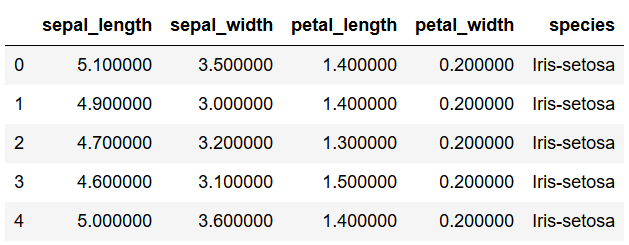
3 Multinomial logistic regression with scikit-learn
First of all we assign the predictors and the criterion to each object and split the datensatz into a training and a test part.
x = iris.drop('species', axis=1)
y = iris['species']
trainX, testX, trainY, testY = train_test_split(x, y, test_size = 0.2)
3.1 Fit the model
Here comes the Multinomial Logistic Regression:
log_reg = LogisticRegression(solver='newton-cg', multi_class='multinomial')
log_reg.fit(trainX, trainY)
y_pred = log_reg.predict(testX)
3.2 Model validation
Let’s print the accuracy and error rate:
print('Accuracy: {:.2f}'.format(accuracy_score(testY, y_pred)))
print('Error rate: {:.2f}'.format(1 - accuracy_score(testY, y_pred)))
Let’s have a look at the scores from cross validation:
clf = LogisticRegression(solver='newton-cg', multi_class='multinomial')
scores = cross_val_score(clf, trainX, trainY, cv=5)
scores
print("Accuracy: %0.2f (+/- %0.2f)" % (scores.mean(), scores.std() * 2))
Let’s have a look at the confusion matrix:
confusion_matrix = confusion_matrix(testY, y_pred)
print(confusion_matrix)
If you have many variables, it makes sense to plot the confusion matrix:
plt.matshow(confusion_matrix, cmap=plt.cm.gray)
plt.show()
3.3 Calculated probabilities
We also have the opportunity to get the probabilities of the predicted classes:
probability = log_reg.predict_proba(testX)
probability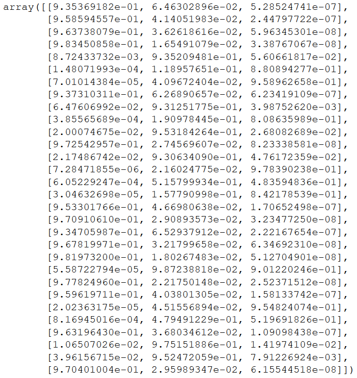
Each column here represents a class. The class with the highest probability is the output of the predicted class. Here we can see that the length of the probability data is the same as the length of the test data.
print(probability.shape[0])
print(testX.shape[0])
Let’s bring the above shown output into shape and a readable format.
df = pd.DataFrame(log_reg.predict_proba(testX), columns=log_reg.classes_)
df.head()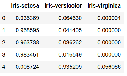
Tip: with the .classes_ function we get the order of the classes that Python gave.
The sum of the probabilities must always be 1. We can see here:
df['sum'] = df.sum(axis=1)
df.head()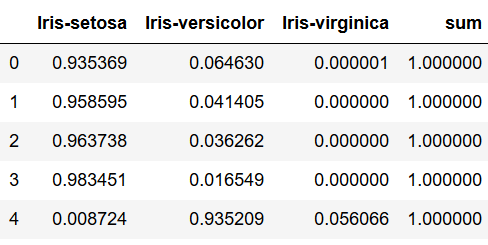
Now let’s add the predicted classes…
df['predicted_class'] = y_pred
df.head()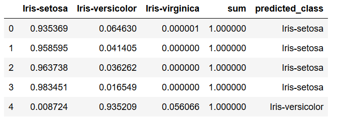
.. and the actual classes:
df['actual_class'] = testY.to_frame().reset_index().drop(columns='index')
df.head()
Now we can do a plausibility check whether the classes were predicted correctly. Unfortunately, the comparison of two object columns works very badly in my test attempts. Therefore I built a small word around in which I convert the predicted_classes and actual_classes using the label encoder from scikit-learn and then continue to work with numerical values.
le = preprocessing.LabelEncoder()

df['label_pred'] = le.fit_transform(df['predicted_class'])
df['label_actual'] = le.fit_transform(df['actual_class'])
df.head()
Here we see that the two variables (predicted_class & actual_class) were coded the same and can therefore be continued properly.
targets = df['predicted_class']
integerEncoded = le.fit_transform(targets)
integerMapping=dict(zip(targets,integerEncoded))
integerMapping
targets = df['actual_class']
integerEncoded = le.fit_transform(targets)
integerMapping=dict(zip(targets,integerEncoded))
integerMapping
Now it’s time for our plausibility check whether the classes were predicted correctly. If the result of subtraction is 0, it was a correct estimate of the model.
df['check'] = df['label_actual'] - df['label_pred']
df.head(7)
For better orientation, we give the observations descriptive names and delete unnecessary columns.
df['correct_prediction?'] = np.where(df['check'] == 0, 'True', 'False')
df = df.drop(['label_pred', 'label_actual', 'check'], axis=1)
df.head()
Now we can use the generated “values” to manually calculate the accuracy again.
true_predictions = df[(df["correct_prediction?"] == 'True')].shape[0]
false_predictions = df[(df["correct_prediction?"] == 'False')].shape[0]
total = df["correct_prediction?"].shape[0]

print('manual calculated Accuracy is:', (true_predictions / total * 100))
Let’s take finally a look at the probabilities of the mispredicted classes.
wrong_pred = df[(df["correct_prediction?"] == 'False')]
wrong_pred
We see we were close to the right class both times.
4 Multinomial Logit with the statsmodel library
To get the p-values of the model created above we have to use the statsmodel library again.
x = iris.drop('species', axis=1)
y = iris['species']
x = sm.add_constant(x, prepend = False)
mnlogit_mod = sm.MNLogit(y, x)
mnlogit_fit = mnlogit_mod.fit()
print (mnlogit_fit.summary())
How to interpret the results exactly can be read “here”.